Model order reduction and component mode synthesis

This section describes the process how to create general flexible multibody system models using the floating frame of reference formulation with model order reduction (here also denoted as CMS). The according object ObjectFFRFreducedOrder is described in Section ObjectFFRFreducedOrder.

Import of flexible bodies

For flexible bodies in multibody systems, specifically for model order reduction, a standard input data (SID) has been defined in the past . A recent formulation for FFRF showed that significantly less information is required for the computation of the dynamics of displacement-based solid finite elements:

• nodal reference positions (given in FEMinterface member variable nodes['Position'])

• stiffness matrix (given in FEMinterface member variable stiffnessMatrix)

• mass matrix (given in FEMinterface member variable massMatrix)

• (given in FEMinterface member variable nodes['Position'])

In addition, the following data may be needed:

• element connectivity: needed for visualization, surface reconstruction and stress computation

• list of surface elements: if not computed internally in Exudyn (stored in FEMinterface member variable surface)

• information on how to obtain stresses from the set of (reduced) coordinates: if not computed internally in Exudyn (stored in FEMinterface member variable postProcessingModes for stresses at nodal positions)

This data can be generated by an appropriate interface to NGsolve:

• FEMinterface.ImportMeshFromNGsolve(...),

or imported from ABAQUS with FEMinterface functions

• ReadMassMatrixFromAbaqus(...),

• ReadStiffnessMatrixFromAbaqus(...),

• ImportFromAbaqusInputFile(...) )

and similar functionality exists for ANSYS. Importing data may be time consuming, which is why all FEMinterface data, including computed modes, can be saved and loaded via SaveToFile and LoadFromFile.

It is assumed that there exists an underlying solid finite element mesh, given by e.g., tetrahedral or hexahedral finite elements. However, this mesh is not needed for computations. If the surface or any part of the flexible body shall be visualized, surface elements (triangles or quads) need to be provided with indices of the mesh nodes. The computation of surface elements is done by FEMinterface function `` VolumeToSurfaceElements``, making use of solid finite elements stored in FEMinterface.elements.

A major advantage of the FEMinterface data is that it is widely independent of underlying finite element technologies, specifically finite element order, reduced integration, etc., however, stress or strain can not be computed as well. A conventional way is to store computed body deformations and perform post processing in the original finite element code, which gives highest quality of stress, strain, and other quantities. A second way is, due to linearity of the small deformation assumptions, to use post-processing modes, such as modes to represent stress components. Post processing modes may be defined in the FEMinterface member postProcessingModes, which is a dictionary containing the modes stored in columns of the matrix, cyclic for every (stress / strain) component and for all modes, and an extra field outputVariableType which denotes the type of modes. The post processing modes may be directly computed in NGsolve with ComputePostProcessingModesNGsolve, using efficient and accurate internal functionality, or calculated with a much slower and very basic Python function ComputePostProcessingModes, which can compute simplified stresses or strains for 4-noded tetrahedral elements.

Eigenmodes

This section will describe the computation of eigenmodes using FEMinterface.

The FEMinterface in the module FEM has various functionality to import finite element meshes from finite element software. We create a FEMinterface by means of

fem = FEMinterface()

which allows us to use the variable fem from now.

Meshes can be imported from NETGEN/NGsolve (Section Class function: ImportMeshFromNGsolve), Abaqus (see Section Class function: ImportFromAbaqusInputFile and other sections related to ABAQUS), ANSYS (see Section Class function: ReadElementsFromAnsys and other sections related to ANSYS). The import procedure, which can also be done manually, needs to include massMatrix \({\mathbf{M}}\) and stiffnessMatrix \({\mathbf{K}}\) from any finite element model. Note that many functions are based on the requirement that nodes are 3D displacement-based nodes, without rotation or other coordinates.

For any functionality with ObjectFFRFreducedOrder and for the computation of Hurty-Craig-Bampton modes as described in the next section, nodesare required. Finally, elements need to be included for visualization, and a surface needs to be reconstructed from the element connectivity, which is available for tetrahedral and hexahedral elements for most import functions.

Fig. 24 Test model and mesh for hinge created with Netgen (linear tetrahedral elements).

As an example, we consider a part denoted as ‘hinge’ in the following, see Fig. 24. The test example can be found in Examples/NGsolveCMStutorial.py with lots of additional features.

After import of mass and stiffness matrix, eigenmodes and eigenfrequencies can be computed using fem.ComputeEigenFrequencies(...), which computes the quantities fem.modeBasis and fem.eigenValues. The eigenvalues in Hz can be retrieved also with the function fem.GetEigenFrequenciesHz(). The function fem.ComputeEigenFrequencies(...) is available for dense and sparse matrices, and uses scipy.linalg to compute eigenvalues of the linear, undamped mechanical system

(22)\[{\mathbf{M}} \ddot {\mathbf{q}}(t) + {\mathbf{K}} {\mathbf{q}}(t) = {\mathbf{f}}(t) .\]

Here, the total number of coordinates of the system is \(n\), thus having the vector of system coordinates \({\mathbf{q}} \in \Rcal^n\), vector of applied forces \({\mathbf{f}} \in \Rcal^n\), mass matrix \({\mathbf{M}} \in \Rcal^{n \times n}\) and stiffness matrix \({\mathbf{K}} \in \Rcal^{n \times n}\). If we are interested in free vibrations of the system, without any boundary conditions or interconnections to other bodies, Eq. (22) can be converted to a generalized eigenvalue problem. Using the approach \({\mathbf{q}}(t) = {\mathbf{v}} \mathrm{e}^{\mathrm{i} \omega t}\) in Eq. (22), and thus \(\ddot {\mathbf{q}}(t) = -\omega^2 {\mathbf{q}}(t)\), we obtain

(23)\[\left[ \left(-\omega^2 {\mathbf{M}} + {\mathbf{K}} \right) {\mathbf{v}} \right] \mathrm{e}^{i\omega t} = \Null .\]

Assuming that Eq. (23) is valid for all times, the generalized eigenvalue problem follows that

(24)\[\left(-\omega^2 {\mathbf{M}} + {\mathbf{K}} \right) {\mathbf{v}} = \Null ,\]

which can be rewritten as

(25)\[\det \left(-\omega^2 {\mathbf{M}} + {\mathbf{K}} \right) = 0 ,\]

and which defines the eigenvalues \(\omega_i^2\) of the linear system, where \(i \in \{0, \ldots, n-1\}\). Note that in this case, the eigenvalues are the squared eigenfrequencies (in rad/s). We can use eigenvalue algorithms to compute the eigenvalues \(\omega_i^2\) and according eigenvectors \({\mathbf{v}}_i\) from Python. The function fem.ComputeEigenmodes(...) uses eigh(...) from scipy.linalg in the dense matrix mode, and in the sparse mode eigsh(...) from scipy.sparse.linalg, the latter being restricted to pure symmetric matrices. Using special shift-inverted techniques in eigsh(...), it performs much better than standard settings. However, you may tune your specific eigenvalue problem by modifying the solver procedure (just copy that function and adjust to your needs). As an output, we obtain the smallest nModes eigenvectors (=eigenmodes)(Eigenvectors are the result of the eigenvalue algorithm, such as the QR algorithm. The mechanical interpretation of eigenvectors are eigenmodes, that can be visualized as shown in the figures of this section.) of the system. Here, we will also use synonymously the terms ‘eigenmodes’ and ‘normal modes’, which result from an eigenvalue/eigenvector computation using certain (or even no) boundary conditions.

Fig. 25 Lowest 8 free-free modes for hinge finite element model, contour plot for \(xx\)-stress component.

Clearly, if there are no supports included in the stiffness matrix, the resulting eigenmodes will contain 6 rigid body modes and we will also call this case for the computation of eigenmodes the free-free case, in analogy to a simply supported beam. This rigid body modes, which are usually not needed (=unwanted) in the succeeding computation, can be excluded with an according option in

fem.ComputeEigenFrequencies(excludeRigidBodyModes = ...)

For our test example, 8 eigenmodes are shown in Fig. 25, where the 6 rigid body modes have been excluded (so in total, 14 eigenvectors were computed). The 8 eigenfrequencies for the chosen coarse mesh with mesh size \(h=0.01\) and 1216 nodes result as

\[f_{0..7} = [ 671.59, 707.17, 1298.50, 1929.97, 1971.76, 3141.47, 3595.34, 4317.51] Hz\]

Note, that a computation with a finer mesh, using mesh size \(h=0.002\) and 100224 nodes, leads to significantly different eigenfrequencies, starting with \(f_0=371.50\,\)Hz. This shows that quadratic finite elements would be more appropriate for this case.

After the computation of modes, it is always a good idea to visualize and/or animate these modes. We can do this, using the function AnimateModes(...) available in exudyn.interactive, which allows us to inspect and animate modes and to create animations for these modes, see the mentioned example.

Clearly, the free-free modes in Fig. 25 are not well suited for the modeling of the deformations within the hinge, if the bolt and the bushing shall be fixed to ground or to another part. Therefore, we can use modes based on ideas of Hurty and Craig-Bampton , as shown in the following.

Hurty-Craig-Bampton modes

This section will describe the computation of static and eigen (normal) modes using FEMinterface. The theory is based on Hurty and Craig-Bampton , but often only attributed to Craig-Bampton. Furthermore, boundaries are also called interfaces(Here, and in the description of various Python functions, we will use boundary and interface often synonymously, as flexible bodies can be either connected to ground in the sense of a classical ‘support-type’ boundary condition, or they can represent the boundary of the flexible body as an interface to joints (via markers).), as they either represent surface sections of our finite element model which are connected to the ground or they represent interfaces to joints and are connected to other bodies.

The computation of so-called static and normal modes follows a simple concept based on finite element mass and stiffness matrices. The final goal of the computation of modes is to approximate the solution \({\mathbf{q}} \in \Rcal^n\)by means of a reduction basis \(\tPsi \in \Rcal^{n \times m}\)and a reduced set of coordinates \({\mathbf{p}} \in \Rcal^m\), for which we assume \(m \ll n\).

In order to include boundary/interface effects, we separate our nodes and the nodal coordinates into

1. boundary nodes \({\mathbf{q}}_b \in \Rcal^{n_b}\) and

2. internal or inner nodes \({\mathbf{q}}_i \in \Rcal^{n_i}\).

We assume that internal nodes are not exposed to boundary/interface conditions or to forces.

Therefore, we may rewrite Eq. (22) as follows

(26)\[\mp{{\mathbf{M}}_{bb}}{{\mathbf{M}}_{bi}}{{\mathbf{M}}_{ib}}{{\mathbf{M}}_{ii}} \vp{\ddot{{\mathbf{q}}}_b}{\ddot{{\mathbf{q}}}_i} + \mp{{\mathbf{K}}_{bb}}{{\mathbf{K}}_{bi}}{{\mathbf{K}}_{ib}}{{\mathbf{K}}_{ii}} \vp{{\mathbf{q}}_b}{{\mathbf{q}}_i} = \vp{{\mathbf{f}}_b}{\Null}\]

or, equivalently,

(27)\[\begin{split}{\mathbf{M}}_{bb} \ddot{{\mathbf{q}}}_b + {\mathbf{M}}_{bi} \ddot{{\mathbf{q}}}_i +{\mathbf{K}}_{bb} {{\mathbf{q}}}_b + {\mathbf{K}}_{bi} {{\mathbf{q}}}_i = {{\mathbf{f}}}_b \\ {\mathbf{M}}_{ib} \ddot{{\mathbf{q}}}_b + {\mathbf{M}}_{ii} \ddot{{\mathbf{q}}}_i +{\mathbf{K}}_{ib} {{\mathbf{q}}}_b + {\mathbf{K}}_{ii} {{\mathbf{q}}}_i = \Null . \label{eq_Guyan_ii}\end{split}\]

A pure static condensation follows from Eq. (26) with the assumption that inertia terms are neglected, leading to the static result for internal nodes,

\[{{\mathbf{q}}}_{i,stat}=-{\mathbf{K}}_{ii}^{-1} {\mathbf{K}}_{ib} {{\mathbf{q}}}_{b} .\]

A pure static condensation, also denoted as Guyan-Irons method, keeps boundary coordinates but removes all internal modes, using the approximation

(28)\[\vp{{\mathbf{q}}_b}{{\mathbf{q}}_i} \approx \vp{{\mathbf{I}}}{-{\mathbf{K}}_{ii}^{-1} {\mathbf{K}}_{ib}} {\mathbf{q}}_b = \tPsi^{GI} {\mathbf{q}}_b ,\]

which leads to no approximations (‘exact’) results for the static case, but poor performance in highly dynamic problems.

Significant improvement result from the Hurty-Craig-Bampton method, which adds eigenmodes of the internal coordinates (internal nodes). We assume that \(\tPsi_{ii}\) is the matrix of eigenvectors as a solution to the eigenvalue problem

(29)\[\left(-\omega^2 {\mathbf{M}}_{ii} + {\mathbf{K}}_{ii} \right) {\mathbf{v}} = \Null ,\]

Hereafter, we will only keep the lowest (or other appropriate) \(m\) eigenmodes in a reduced eigenmode matrix,

\[\tPsi^{(red)}_{ii} = \left[\tPsi_{ii,0}, \ldots, \tPsi_{ii,m-1} \right]\]

Combining these ‘fixed-fixed’ eigenvectors with the Guyan-Irons reduction (28), we obtain the Hurty-Craig-Bampton modes as

\[\vp{{\mathbf{q}}_b}{{\mathbf{q}}_i} \approx \vp{{\mathbf{I}}}{-{\mathbf{K}}_{ii}^{-1} {\mathbf{K}}_{ib}} {\mathbf{q}}_b + \vp{\Null}{\tPsi_{r,i}} {\mathbf{p}}_{r} ,\]

or in matrix form

(30)\[\vp{{\mathbf{q}}_b}{{\mathbf{q}}_i} \approx \mp{{\mathbf{I}}}{\Null}{-{\mathbf{K}}_{ii}^{-1} {\mathbf{K}}_{ib}}{\tPsi_{r,i}} \vp{{\mathbf{q}}_b}{{\mathbf{p}}_r} = \tPsi^{HCB} {\mathbf{p}}^{HCB} .\]

The disadvantage of Eq. (30) is evident by the fact that there may be a large number of boundary/interface nodes, leading to a huge number of static modes (100s or 1000s) and thus making the model reduction inefficient. Therefore, we can switch to other interfaces, as described in the following.

Definition of RBE2 / RBE3 interfaces

A powerful extension, which is available in many finite element as well as flexible multibody codes, is the definition of special boundary/interface conditions, based on pure rigid body motion. The so-called RBE2 boundaries are defined such that they are firmly connected to a rigid frame, thus the boundary or interface can only undergo rigid body motion. The advantage of this procedure is that, in comparison to Eq. (30), the number of boundary/interface modes is given by 6 rigid body modes, which allow simple integration into standard joints of multibody systems, e.g., the GenericJoint. The disadvantage is that such modes usually lead to artificial stiffening and stresses close to the boundary.

For so-called RBE3 boundaries, the kinematics is significantly different. The displacement of RBE3 boundaries is the (weighted) average displacement of all boundary nodes. The resulting forces at the RBE3 boundary are equally distributed, again using node-weighting. The (linearized) rotation of RBE3 boundaries is computed as the weighted displacements of the boundaries and including the distance to the rotation axes. Forces due to torques at RBE3 boundaries are computed according to the weighting, again considering the distance to the rotation axes, see the according formulas later on. The computation of RBE3 boundaries widely follows the formulation of the MarkerSuperElementRigid, see Section MarkerSuperElementRigid.

Computation of Hurty-Craig-Bampton modes with RBE2 interfaces

In the following section, we show the procedure for the computation of static modes for the RBE2 rigid-body interfaces. Note that eigenmodes directly follow from matrices \({\mathbf{M}}_{ii}\) and \({\mathbf{K}}_{ii}\) as described in Section Hurty-Craig-Bampton modes. The implementation is given in fem.ComputeHurtyCraigBamptonModes(...), see Section Class function: ComputeHurtyCraigBamptonModes.

First, we use the index \(j\) here as a node index, having the clear correspondence to the coordinate index \(i\), that node \(j\) has coordinates \([3\cdot j,\; 3\cdot j+1,\; 3\cdot j+2]\). Furthermore, nodes are split into boundary and internal nodes, which then leads to according internal and boundary coordinates. We shall note that this sorting is never done in the finite element model or matrices, but just some indexing (referencing) lists are generated and used throughout, using valuable features of numpy.linalg and scipy.sparse.

For a certain boundary node set \(B=[j_0, \; j_1, \; j_2, \; ...] \in \Ncal^{n_b}\) with certain \(n_b\) node indices \(j_0, ...\), we define one boundary set. The following transformations need to be performed for every set of boundary node lists. We also assume that weighting of all boundary nodes is equal, which may not be appropriate in all cases.

If we assume that there may only occur rigid body translation and rotation for the whole boundary node set, which is according to the idea of so-called RBE2 boundary conditions, it follows that the translation of all boundary nodes is given by

\[{\mathbf{T}}_t = \vr{ {\mathbf{I}} }{ \vdots}{ {\mathbf{I}}} \in \Rcal^{3 n_b \times 3}\]

with \({\mathbf{I}} \in \Rcal^{3\times 3}\) identity matrices. The nodal translation coordinates on boundary \(B\) are denoted as \({\mathbf{q}}_{B,t} \in \Rcal^3\). The translation of the boundary/interface is mapped to the boundary coordinates as follows (assuming only one boundary \(B\)),

\[{\mathbf{q}}_{b,t} = {\mathbf{T}}_t \, {\mathbf{q}}_{B,t}\]

The nodal rotation coordinates on boundary \(B\) are denoted as \({\mathbf{q}}_{B,r} \in \Rcal^3\). The rotation of the boundary/interface is mapped to the boundary coordinates as follows (assuming only one boundary \(B\)),

\[{\mathbf{q}}_{b,r} = {\mathbf{T}}_r \, {\mathbf{q}}_{B,r}\]

The computation of matrix \({\mathbf{T}}_r\) is more involved. It is based on nodal (reference) position vectors \({\mathbf{r}}^{(0)}_j\), \(j \in B\), the midpoint of all boundary nodes,

\[{\mathbf{r}}^{(m)} = \frac{1}{n_b} \sum_{j=0}^{n_b-1} {\mathbf{r}}^{(0)}_j\]

and the position relative to the midpoint, denoted as

\[{\mathbf{r}}_j = {\mathbf{r}}^{(0)}_j - {\mathbf{r}}^{(m)} .\]

Note that the coordinate system refers to the system used in the underlying finite element mesh. The transformation for rotation follows from

\[{\mathbf{T}}_r = \vr{ \tilde {\mathbf{r}}_0 }{ \vdots}{ \tilde {\mathbf{r}}_{n_b-1}} \in \Rcal^{3 n_b \times 3} .\]

The total nodal coordinates at the boundary, representing translations and rotations, follow as

\[{\mathbf{q}}_{B} = \vp{{\mathbf{q}}_{B,t}}{{\mathbf{q}}_{B,r}} ,\]

and the transformation matrix for the translation and rotation simply reads

\[{\mathbf{T}} = [{\mathbf{T}}_t \;\; {\mathbf{T}}_r] \in \Rcal^{3n_b \times 6} ,\]

which provides the total mapping of boundary rigid body motion

\[{\mathbf{q}}_{b} = {\mathbf{T}} \, {\mathbf{q}}_{B} ,\]

which is the sum of translation and rotation.

As an example, having the boundary nodes sorted for two boundary node set \(B_0\) and \(B_1\), we obtain the following transformation for the Hurty-Craig-Bampton method with only 6 modes per boundary node set,

(31)\[\vp{{\mathbf{q}}_b}{{\mathbf{q}}_i} \approx \mr{ {\mathbf{T}}_0}{\Null}{\Null} {\Null}{{\mathbf{T}}_1}{\Null} {-{\mathbf{K}}_{ii}^{-1} {\mathbf{K}}_{ib}\vp{{\mathbf{T}}_0}{\Null} }{-{\mathbf{K}}_{ii}^{-1} {\mathbf{K}}_{ib}\vp{\Null}{{\mathbf{T}}_1} }{\tPsi_{r,i}} \vr{{\mathbf{q}}_{B_0}}{{\mathbf{q}}_{B_1}}{{\mathbf{p}}_r} .\]

with the new boundary node vector \({\mathbf{q}}_b = [{\mathbf{q}}_{B_0}\tp \;\; {\mathbf{q}}_{B_1}\tp]\tp\).

Notes:

• The inverse \({\mathbf{K}}_{ii}^{-1}\) is not computed, but this matrix is LU-factorized using sparse techniques.

• The factorization only needs to be applied to six vectors for every relevant boundary node set.

• One set of boundary nodes can be omitted from the final static modes in Eq. (31), because keeping all boundary modes, would introduce six rigid body motions to our mode basis, what is usually not wanted nor needed.

Using again the examples given in Fig. 24, we now obtain a set of modified modes using the function fem.ComputeHurtyCraigBamptonModes(...). Fig. 26 shows the first 6 rigid body modes. Note that these modes are automatically removed in the function fem.ComputeHurtyCraigBamptonModes(...) with default settings. Fig. 27 shows the second set of 6 rigid body modes. Finally, 8 eigenmodes have been computed for the fixed-fixed case (where all boundary/interfaces nodes are fixed), see Fig. 28. The eigenfrequencies for this case now are significantly higher than in the free-free case, reading

\[f_{0..7} = [1277.35, 1469.86, 3336.91, 3584.28, ...]\]

Fig. 26 Static modes for bolt rigid body interface, using Hurty-Craig-Bampton method; top three images show (x,y,z)-translation modes, bottom three images show (x,y,z)-rotation modes; contour color represents norm of displacements.

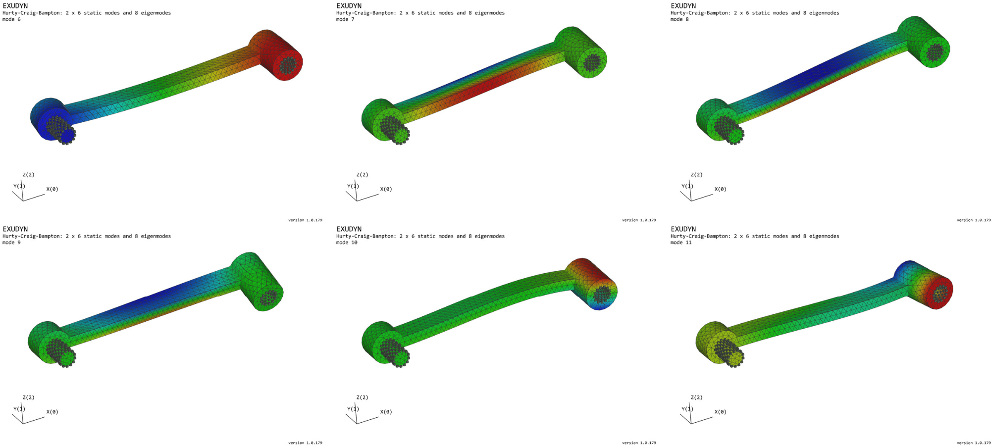
Fig. 27 Static modes for bushing rigid body interface, using Hurty-Craig-Bampton method; top three images show (x,y,z)-translation modes, bottom three images show (x,y,z)-rotation modes; contour color represents norm of displacements.

Fig. 28 Eigenmodes for fixed-fixed case, resulting from Hurty-Craig-Bampton method; contour color represents norm of displacements.

Computation of Hurty-Craig-Bampton modes with RBE3 interfaces

we are currently finishing a paper, after which this section will be completed!

Computation of stresses and strains for CMS modes

The computation of stresses and strains is not directly possible if only knowing nodal displacements, stiffness matrix and mass matrix. In the following, we assume that we have a vector of nodal displacements \({\mathbf{q}}\), reduced coordinates \({\mathbf{p}}^{R}\), as well as a reduction matrix \(\tPsi^{R}\), compare Eq. (30),

(32)\[{\mathbf{q}} \approx \tPsi^{R} {\mathbf{p}}^{R} .\]

Knowing all nodal displacements of a finite element allows to compute displacement, stress, and strain field within the element. This procedure is usually done within the finite element codes. In particular, one should know that stress and strain quantities are having a lower order of accuracy than displacements and they may be more accurate in certain points, e.g., integration points. Furthermore, stress and strain quantities may have jumps along element boundaries, which is why they are usually post-processed in order to at least look smoother but in general also are more accurate.

In Exudyn, we have the option to pre-compute stress or strain components at finite element nodes, see the options below. Due to the fact that the FFRF / CMS formulation is assuming small (linearized) strains only, we are able to superimpose stress and strain for each mode. Independently of the quantity we intend to compute (stress, strain or similar), we use post-processing modes, which allow to represent special output variables.

Having a modal coordinate \({\mathbf{p}}^{R}_k\), we define a post-processing mode (pm) such that

\[{\mathbf{s}}_k^{\mathrm{pm}} = \tPsi^{\mathrm{pm}}_k {\mathbf{p}}^{R}_k ,\]

in which \({\mathbf{s}}_k^{\mathrm{pm}}\) represents for example the stress component \(\sigma_\mathrm{xx}\) for the mode \(k\). Putting together all stress modes for \(\sigma_\mathrm{xx}\), \(\sigma_\mathrm{yy}\), \(\sigma_\mathrm{zz}\), \(\sigma_\mathrm{yz}\), \(\sigma_\mathrm{xz}\), and \(\sigma_\mathrm{xy}\),

\[\tPsi^{\sigma_\mathrm{xx}} = \left[\tPsi^{\sigma_\mathrm{xx}}_0, \tPsi^{\sigma_\mathrm{xx}}_1, \ldots, \tPsi^{\sigma_\mathrm{xx}}_{m-1}\right] ,\]

we are able to compute \(\sigma_\mathrm{xx}\) for all nodes from the relation

\[{\mathbf{s}}^{\sigma_\mathrm{xx}} = \tPsi^{\sigma_\mathrm{xx}} {\mathbf{p}}^{R}\]

Using the FEMinterface member postProcessingModes, the FEM module, we can define the matrix as \(\tPsi^{\sigma_\mathrm{ij}}\) for every node of the finite element mesh. In particular, one has to store all stress (or strain) components consecutively for each mode, which means that for mode \(k\), \(\tPsi\) contains the columns

\[\tPsi^{\sigma}_k = \left[\tPsi^{\sigma_\mathrm{xx}}_k, \tPsi^{\sigma_\mathrm{yy}}_k, \tPsi^{\sigma_\mathrm{zz}}_k, \tPsi^{\sigma_\mathrm{yz}}_k, \tPsi^{\sigma_\mathrm{xz}}_k, \tPsi^{\sigma_\mathrm{xy}}_k\right] ,\]

For more details, see the FEM module in Section Class function: __init__, either for function ComputePostProcessingModes or ComputePostProcessingModesNGsolve.

In order to retrieve modes, we currently have three options:

• Re-compute stress or strain quantities for given material parameters from nodal displacements for linear tetrahedral elements (Tet4), using the function ComputePostProcessingModes within the FEM module. This function is implemented in Python and therefore comparatively slow.

• For NGsolve models, you can use the ComputePostProcessingModesNGsolve, which takes the finite element space and material to compute post-processing modes directly in NGsolve, which is comparatively fast, if you do not have an excessive amount of modes and nodes.

• You can compute the post-processing modes within your finite element tool, such as Ansys or Simulia(ABAQUS) and import them manually. There exists no functionality in Exudyn to do so.

In general, one should know that the size of postprocessing modes may be huge. If you have \(200\,000\) nodes and 100 modes, the matrix \(\tPsi^{\sigma}\) would have the size \(200\,000 \times (6 \cdot 100)\), thus leading to \(120\,000\,000\) components, close to 1GB of memory. In other words, it could make sense to consider computation of stresses in a post-computing phase.

Interfaces and boundaries

Being able to model a sole flexible body is not sufficient for the modeling of industrial problems. An important part of component mode synthesis is the appropriate definition of boundaries or interfaces. The term interface is widely used and may be more appropriate when connecting two bodies via such interfaces. However, in some cases the flexible body may be fixed to ground via such a boundary. In order to distinguish boundary/interface (b) and internal nodes (i), boundary seems to be appropriate and boundary/interface will be used synonymously in the context of flexible bodies.

An boundary/interface is represented by a certain surface area of a body, usually defined by surface elements and underlying nodes. For simplicity, it may just be defined by means of a node set. This is sufficient, in order for most of the previously described algorithms to work. If node sets are not imported from the underlying finite element codes, practical functions exist for the definition of node sets from geometrical operations, specifically(Note that these functions perform a linear search in the whole mesh, which is computationally inefficient if it is called many times.):

• GetNodeAtPoint: returns node number of a single node (if found) at given spatial position, with certain tolerance

• GetNodesInPlane: returns all nodes lying on a defined plane with certain tolerance

• GetNodesInCube: returns all nodes lying in a axis-parallel cube

• GetNodesOnLine: returns all nodes lying on a line defined by two points, with certain tolerance

• GetNodesOnCylinder: returns all nodes lying on a cylinder defined by two points and radius, with certain tolerance

• GetNodesOnCircle: returns all nodes lying on a circle defined by point, normal and radius, with certain tolerance

In order to compute according weighting factors, surface elements need to exist, either importing them the finite element code, or by using the FEMinterface member surface. The surface of tetrahedral or hexahedral meshes, which follow a standard node numbering, can be computed using the FEMinterface function VolumeToSurfaceElements.

Node weighting

As mentioned in the literature , there are certain advantages to use regular meshes on boundaries/interfaces. However, industrial relevant geometries often cannot be meshed by regular hexahedral meshes which leads to unstructured tetrahedral elements with (nearly) arbitrary triangular surfaces. While being a more general approach, an according nodal weighting is inevitable for unstructured surface meshes. As a drawback, accurate nodal weighting for application of forces or for computation of average displacements or rotations requires the information of underlying finite element interpolation functions, which are avoided in the present approach. A simplified, first order accurate functionality is provided by GetNodeWeightsFromSurfaceAreas, which reconstructs nodal weights for a set of node numbers from a given triangulated surface in FEMinterface. After identification of surface triangles and computation of according triangle areas, the weight \(w_i\) of every node \(i\) is built upon the according area of all connected triangles \(j\),

\[w_i = \frac{1}{3 A_B} \sum_{j} A_j , \quad \mathrm{and} \quad \sum_i w_i = 1\]

using the total area \(A_B\) of the boundary. This weighting leads to nearly constant strain distribution along the cross section of a fixed bar with equally distributed axial forces.

Reference conditions

Currently, there is no specific functionality to define reference conditions for FFRF objects in Exudyn. In the ObjectFFRF, a ObjectConnectorCoordinateVector needs to be used to define constraints of a so-called Tisserand frame.

In the ObjectFFRFreducedOrder, there are in general two approaches:

• The computed modes do not include rigid body motions, by using the appropriate flagexcludeRigidBodyModes = Truefor most of such functions; in this case, the reference conditions are defined such that the reference node positions of the mesh are rigidly attached to the reference frame. In case of Hurty-Craig-Bampton modes, one boundary set (the first one) is attached to the reference frame.

• Alternatively, excludeRigidBodyModes can be set False, or arbitrary modes can be imported from elsewhere.

  In this case, rigid body motion must be excluded by appropriate constraints, e.g., a ObjectConnectorCoordinateVector applied to the NodeGenericODE2 of ObjectFFRFreducedOrder. This task is completely left to the user.

It should be noted that regarding efficiency or highest accuracy, better reference conditions may exists, which are not fully supported in the current code and may only be applied with user functions.

For further information on this topic read: theDoc.pdf