Introduction to multibody systems
The intention of the subsequent sections is to give brief introductions into subjects which are essential for working with multibody systems. Some of the contents may not go deep enough, which is why we refer to the according literature. In particular, the contents follow the books of
Woernle , Multibody Systems, 2024
A.A. Shabana , Dynamics of Multibody Systems, 2014
P.E. Nikravesh , Computer-Aided Analysis of Mechanical Systems, 1988
Multibody systems are mechanical systems of bodies (sometimes only one body), which are interconnected. Multibody systems may include linear dynamical systems as used in vibration analysis and rotordynamics. However, multibody systems are often characterized by nonlinear and differential-algebraic equations, and they typically cover arbitrary rigid body motions. In a broader sense, multibody systems represent the mechanical part of mechatronics systems. The range of multibody systems might vary from simple one or two-mass oscillators, or single or double pendulums, up to complex full-scale vehicles or aerospace systems.
Multibody systems (MBS) are characterized by rigid or flexible bodies that are interconnected by means of joints, contacts, springs and dampers and usually driven by electrical, hydraulic or pneumatic actuators, and possibly subject to external forces. Sophisticated models of joints include the deformation of the joint surface and consider contact and friction models.
Historical development
The roots of analysis tools for multibody systems trace back to Newton’s laws and Euler’s contributions to the motion of rigid bodies. Lagrange introduced a formalism to derive the equations of motions for complex rigid or flexible multibody systems, which is still state of the art. Multibody system dynamics attracted the attention of engineers as soon as computer power was large enough to simulate the nonlinear dynamic behavior of such systems numerically, however only using ordinary differential equations for modeling in the beginning. Since the 1960s, flexibility of structures has been introduced, e.g., in order to understand the instability of a satellite with flexible antennas or a helicopter’s rotor blades. Since the 1990s flexible multibody system methods have been applied in vehicle and aerospace industry, in particular because model order reduction became available and real life components could be simulated. Models where mainly made out of kinematic trees, using minimum coordinate models in the beginning. For long time, algebraic constraints could only be approximated, such as with Baumgarte’s stabilization introduced in the 1970. Major advances on differential-algebraic solvers have been made in the 1990s, introducing Raudau-5 of Hairer and Wanner, as well as BDF solvers of Linda Petzold. Because both approaches had drawbacks, the implicit generalized-alpha solver (Chung, Hubert; Arnold, Brüls) has become a quasi-standard in the 2000s, as it allows to solve almost any index 3 (position level) constraint problem with high efficiency.
Simulation tools in computational engineering
As in Exudyn, the main intention is to create computer models for mechanical systems. The further analysis of the system is left to the users’ needs. In particular, engineers are interested in
(Forward) dynamic analysis:
Dynamic simulation, by setting initial conditions and using time integration for the equations of motion of the model
Outputs may be displacements, rotations, velocities, angular velocities, accelerations, stresses, joint or support forces, etc.
(Forward) static analysis:
(Nonlinear) static computation, by solving the equations of motion without inertia forces and without time-dependency (usually settings accelerations and velocities to zero, but possibly also computing quasi-static or stationary solutions)
Outputs may be displacements, rotations, stresses, joint or support forces, etc.
Kinematic analysis:
Similar to a static analysis, inertia forces are neglected, and in addition forces are neglected as well.
Inputs may be prescribed translations or rotations to specific bodies or joints.
Outputs may be ratios of angular velocities, or the motion of bodies due to prescribed motion in specific joints
Analysis of a multibody system
Kinematic analysis regarding system degree of freedom (DOF), redundant constraints, jacobians (e.g., how joint velocities affect velocities of a particular body)
Critical loads (buckling and bifurcation)
Eigenfrequency and eigenmode analysis
Instability analysis (e.g. critical velocity of trains, fluids, etc.)
Inverse static and dynamic analysis
Computation of required loads in order to reach certain displacements
Inverse kinematics: computation of joint angles of robots in order to obtain a certain tool-center position
Inverse dynamics: computation of joint forces to compensate weight and inertia forces of robot mechanism under motion
Optimization
Minimization of maximum stress within bodies, or of stress to yield-stress ratio
Optimizing kinematic behavior
Minimization of energy
Minimization of damage and wear
Sensitivity analysis
Investigate the influence of small variations of the parameters (dimensions, material, etc.) on the measured values, such as displacements, forces, etc.
Realtime simulation
Hardware-in-the-loop simulation: e.g. in virtual reality, the user acts in reality, while the machine input and feedback is simulated in realtime.
Software-in-the-loop simulation: while the real machine, or parts of it, are considered, other hardware, controllers or humans are emulated by software.
Components of a multibody system
Any multibody system basically consists of a set of components, each of which with specific properties and dependencies. Main components are:
Bodies:
mass points
rigid bodies
flexible bodies (in general)
finite elements (often representing flexible bodies)
Connectors:
spring-dampers (bushings)
joints (represented by algebraic equations)
general constraints (such as on coordinates)
Further components are:
Loads: forces, moments, body loads, gravity, applied to bodies; loads are usually not coupled to the motion of bodies, as compared to springs; however, follower loads may depend on body rotation. Loads may be time-dependent, which can be realized by defining a load together with a user function, or prescribing a load in each time step.
Sensors: measure displacements, velocities, stresses, strains, bending moments, loads, etc., and the do not affect the system behavior, as long as the are not used in controllers or control units.
graphical representation for bodies and system components
Joint control: certain feed-back control laws (e.g., PID) for each joint axis, in order to prescribe joint rotation, velocity, etc., which may in particular result in coupling of system equations.
Motion control, path planning: prescribing a desired path for one or several joints, using a feed-forward control
Control units: controlling the behavior of the system (such as a sequence of tasks, feeding a list of motion control tasks for several joint axes); often realized as scripts
Kinematics basics
Kinematics, also referred to as the geometry of motion, is a fundamental aspect of multibody systems that focuses on the description of motion without considering the forces that cause it. It involves the study of the positions, velocities, and accelerations of body parts in a system and how these quantities change over time. For rigid bodies or bodies that employ frames, it also includes rotations, angular velocities and angular accelerations. This branch of mechanics provides the essential framework for understanding how individual components of a multibody system move relative to one another, laying the groundwork for the subsequent analysis of dynamics where forces are taken into account.
Kinematics is also related to to trajectories (including frames co-moving along trajectories), curve length, motion of frames, and homogeneous transformations. Kinematic constraints are used to define joints, basically by constraining specific relative motion, such as the distance between two particles, the relative rotation or the relative translation along axis. For non-holonomic constraints, the constraint equations have to be defined at velocity level, such as the idealized rolling (wheel) or slipping conditions (sled skid).
Kinematic synthesis involves designing a mechanism’s geometry, including its links and joints, to achieve specific motions. In contrast, kinematic analysis focuses on determining the kinematic quantities, such as positions, velocities, and accelerations, of certain points or components within a mechanism that is performing a prescribed motion.
Links, joints, kinematic chains and trees
Kinematics has been studied much earlier than the development of multibody system dynamics. Traditionally in kinematics, joints were the essential part to define specific (relative) motion. The various joints in a system were linked by “links“, which had no further role in the geometry of motion, without consideration for forces or inertia. However, with advancements in the field of rigid and flexible multibody dynamics, the significance of links has been elevated, and they are more commonly referred to as bodies, considering their dynamic properties.
A series of interconnected links forms a kinematic chain. In most mechanisms, except for those designed for flight, at least one link is stationary, serving as a reference point or frame for the system. This stationary link is typically referred to as the ground or frame. Mechanisms can be classified based on the motion of their links: if all links move within a single plane, the mechanism is called a planar mechanism; otherwise, it is known as a spatial mechanism.
It is also crucial to differentiate between open-loop and closed-loop mechanisms. An open-loop mechanism is characterized by a configuration where traversing through the links in sequence does not lead back to the starting point. In the general case, such an open-loop system is represented by a kinematic tree, which has a root link, and every link can have arbitrary many joints – as long as it leads to no single closed loop. Conversely, a closed-loop mechanism features a configuration where at least one path forms a loop, including the ground link, allowing for the possibility of returning to the starting link through the sequence of connections.
Fig. 15a shows a double pendulum, which is an example of an open-loop mechanism. A closed-loop mechanism is shown in Fig. 15b, which is a four-bar linkage. As mentioned before, the fourth link is the ground link.

Fig. 15 a.) Open loop mechanism (double pendulum), b.) Closed loops mechanism (four-bar linkage).
Kinematic pairs
During early achievements in kinematics, joints have been denoted as kinematic pairs, where the pair represents two bodies where joint constraints are imposed at. There are joints denoted as lower pairs, which are defined by the idealized contact of two rigid surfaces, each of which attached to one of the two bodies. The most prominent types, with mention of the respective object names in Exudyn, are:
spherical joint (S), ball and socket joint; three constraints on relative translation of body-fixed points;
ObjectJointSphericalrevolute (R) joint, hinged joint; three spherical joint constraints plus two on tilting around axes normal to the joint axis;
ObjectJointRevoluteprismatic (P) joint; tree constraints on relative rotation;
ObjectJointPrismaticscrew (helical, H) joint;
not yet availablecylindrical (C) joint;
ObjectJointGenericplanar joint; restricts motion to plane, thus adding one relative translation and two rotation constraints;
ObjectJointGeneric
A very practical joint, which has no relevance for kinematics, is the rigid joint (6 constraints, ObjectJointGeneric). It simply constrains the rigid body motion of two bodies, making the two bodies identical from the rigid body kinematics viewpoint.
Higher pairs involve changing surfaces or curves of contact, such as in a cam and follower or gears.
Indeed, some cases in constraints may not be represented by a set of kinematic pairs, such as several mass points arranged along an inextensible string. Therefore, codeName usually employs kinematic pairs, but also allows an arbitrary number of bodies to be coupled.
Euler’s and Chasles’s Theorems
In the following, we consider so-called active rotations of bodies. Consider a body rotating with an angular velocity \(\tomega\). Thereing, the orientation of the body can be given with respect a previous orientation using a transformation matrix (rotation matrix). Here, the components of the transformation matrix are given as a function of time. When reconsidering the DOF of a mechanism, it is thus the question, how many independent coordinates are required to describe a spatial rotation?
The answer to this question is given by Euler’s theorem:
Euler’s theorem: The general displacement of a body with one point fixed is a rotation about some axis.
The latter theorem states that at any current time \(t\) and after any rotations, the orientation of the body can be described by a rotation axis and a single rotation angle. Note that this rotation axis is used to describe the rotation of the body from the initial to the current time at once, although, the rotation might have been performed by means of many different successive rotations. This rotation axis is different from the so-called instantaneous axis of rotation of the body. As a consequence, points lying at the rotation axis are not affected by this rotation.
In addition to Euler’s theorem, we mention Chasles’s theorem, which reads as follows:
Chasles’s theorem: The most general displacement of a body is a translation plus a rotation.
Therefore, the general motion of the rigid body follows from Euler’s theorem plus a translation of the point which was originally fixed.
Degree of freedom – DOF
According to Nikravesh, “The minimum number of coordinates required to fully describe the configuration of a system is called the number of degrees of freedom of the system”. We may consider two examples given in Fig. 16, to understand the DOF. A double pendulum is shown, which can be described with no less than two independent angles \(\phi_1\) and \(\phi_2\), thus the system has two degrees of freedom.
As a second example, a four-bar mechanism is shown, see Fig. 16b. There are three angles \(\phi_a\), \(\phi_b\) and \(\phi_c\) related with the current configuration of the system. However, there are two algebraic relations (constraint conditions) between these three angles, given as
In the latter two equations, the angles \(\phi_a\) and \(\phi_b\) can be expressed in terms of \(\phi_c\). Thus, \(\phi_c\) is the only remaining independent (minimum) coordinate of the system, and as a consequence, the system has only one degree of freedom. Regarding the four-bar mechanism, there exist some configurations, which can lead to bifurcation and a change in the degrees of freedom – but this is usually avoided in practical cases.
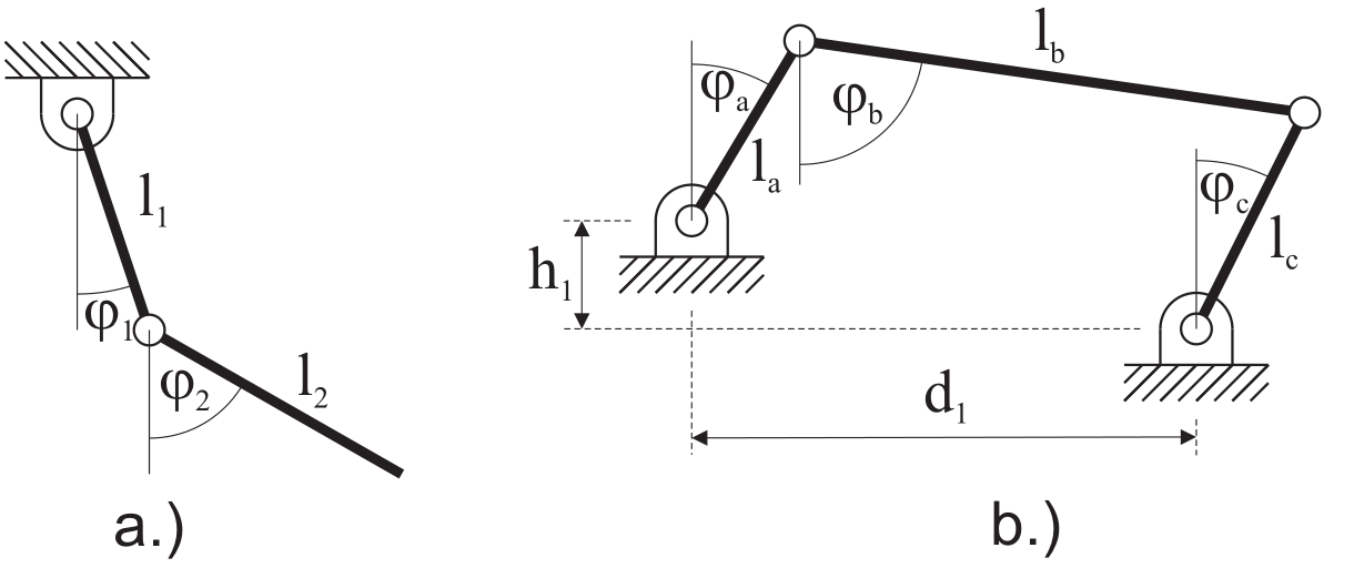
Fig. 16 Examples of mechanisms with different degrees of freedom.
Non-holonomic constraints
It should be noted, that the above given definition works well with holonomic constraints. In case of non-holonomic systems, the non-holonomic constraints, which may only be given at velocity level, lead to different degrees of freedom on position and velocity level. Due to the fact that time integration integrates velocities and accelerations, and constraints may be formulated on position or velocity in Exudyn, non-holonomic constraints are not largely influencing the structure of the system of equations. However, in view of the constraint jacobian, it usually reflects the constraints on velocity level, as this is the matrix which the incremental solver uses to update coordinates.
Dependent and independent coordinates
Assuming a holonomic mechanical system with \(k\) degrees of freedom, one can find \(k\) independent coordinates (minimum coordinates) to completely describe the system configuration. Note that these coordinates do not necessarily have the meaning of displacement, length or angle, but they may be more general (generalized coordinates).
In addition to the independent coordinates, there may be dependent coordinates, similar to the angles \(\phi_a\) and \(\phi_b\) which are dependent on \(\phi_c\) in the example of the four-bar mechanism. It is left to the engineer, whether to find the minimum coordinates of a system and to write all equations in terms of these, or to work with a larger set of independent and dependent coordinates together with algebraic constraint conditions.
Chebychev-Grübler-Kutzbach criterion
A rigid body in space has six degrees of freedom, and thus, six independent coordinates can be used to describe its configuration. Thus for a system with \(n_b\) bodies, there are \(6 \cdot n_b\) coordinates, to describe the bodies. Assuming that there are a set of spheric, revolute, prismatic and other joints, which reduce the degrees of freedom, we denote the number of independent constraints to be of size \(n_c\). It is important, that the constraint equations are (linearly) independent, because in kinematics it is possible to restrict the motion with redundant constraints, see later.
Finally, having \(n_b\) rigid bodies \(n_c\) scalar, independent constraint equations, the degrees of freedom are given as
which is denoted sometimes as the Kutzbach, or Chebychev-Grübler-Kutzbach criterion.
In the case of planar mechanisms, a body obtains only three degrees of freedom. Therefore the Chebychev-Grübler-Kutzbach criterion reads
As a spatial example, consider again the double pendulum Fig. 16a as a spatial mechanism. In this case, there are two bodies, \(n_b=2\) and two revolute joints with 5 constraints each, giving \(n_c=10\). Thus, the Chebychev-Grübler-Kutzbach criterion gives \(n_\mathrm{DOF} = 12 - 10 = 2\), which we expect.
As another example, consider a spatial four-bar mechanism according to Fig. 16b. In this case, there are four bodies, \(n_b=4\), four revolute joints with 5 constraints each and a ground joints with 6 constraints, totalling at \(n_c=4\cdot 5 + 6 = 26\). Thus, Eq. (2) gives
This is certainly not what we expect, as we know that the mechanism can move and has \(n_\mathrm{DOF} = 1\). The reason for this number lies in redundant constraints, which may not be counted for the Chebychev-Grübler-Kutzbach criterion. A solution to this problem is to replace one revolute joint by a planar revolute joint (2 constraints), which then gives
Therefore, Exudyn uses an extended Chebychev-Grübler-Kutzbach criterion for redundant constraints,
where \(n_r\) is the number of redundant constraints and \(n_\mathrm{ODE2}\) is the number of ODE2 coordinates, which may be \(6 \cdot n_b\) for purely spatial rigid bodies, \(n_{ca}\) are pure algebraic constraints and \(n_r\) are redundant constraints.
In Exudyn, there is a function ComputeSystemDegreeOfFreedom in the solver module, available as
mbs.ComputeSystemDegreeOfFreedom(verbose=True)
which allows to compute ODE2 coordinates (\(=n_\mathrm{ODE2}\)), total constraints (\(=n_c\)), redundant constraints (\(=n_r\)), and the degree of freedom (\(=n_\mathrm{DOF}^*\)). In addition, the function also computes the number of pure algebraic constraints (\(=n_{ca}\)), which are internal constraints, which only act on the algebraic quantities but do not affect ODE2 coordinates.
As an example for pure algebraic constraints, in a GenericJoint inactive constraints are replaced by \(\lambda_i=0\) (\(\lambda\) being the Lagrange multiplier), thus reducing the number of effective constraints in the system.
Generalized coordinates
In Cartesian coordinates, three parameters (denoted as coordinates) are used to uniquely define the position of any point with respect to a Cartesian coordinate system. The position and orientation of a rigid body can be uniquely defined by means of three position and three rotation parameters (rigid body coordinates).
The position and orientation as well as the deformation in deformable bodies can be defined by a set of coordinates. We require that any set of coordinates uniquely defines the position of all points of the bodies. As the bodies move, the coordinates vary with time. The set of \(n\) generalized coordinates is commonly represented by a (column) vector
in which \(n\) represents the total number of coordinates that are used. In Exudyn, position, orientation and deformation coordinates (of bodies) are denoted as ODE2 coordinates, as they are related to second order differential equations, the main criterion to distinguish computational coordinates in the system.
The generalized (Lagrangian) coordinates, which are employed in Lagrange’s equations of motion, are another set of well known coordinates used for mechanisms. As known from Lagrange’s formalism, coordinates may be defined relative to each other.
Reference and current coordinates
An important fact on the coordinates used in Exudyn is upon the additive(This additive splitting is also used for rotations: therefore, only the sum of reference and current (or visualization) coordinates has a geometrical meaning, while the parts are only used within the solver for incrementing.) splitting of quantities (e.g. position, rotation parameters, etc.) into reference and current (initial/visualization/…) coordinates. The current position vector of a point node is computed from the reference position plus the current displacement, reading
In the same way rotation parameters are computed from,
which are based on reference quantities plus displacements or changes. Note that these changes are additive, even for rotation parameters. Needless to say, \(\tpsi\cCur\) do not represent rotation parameters, while \(\ttheta\cRef\) should be chosen such that they represent the orientation of a node in reference configuration.
The necessity for reference coordinates originates from finite elements, which usually split nodal position into displacements and reference position.
However, we also use the reference position here in order to define joints, e.g., using the utility function CreateRevoluteJoint(...).
Note that this splitting is only employed for position coordinates, but not for velocities, accelerations or special coordinates. See also Section Reference coordinates and displacements.