Frames, rotations and coordinate systems

In this section, we introduce frames, which provide reference points and rotations attached to the ground or to bodies, thus providing a bases for coordinate systems.

Reference points and reference frames

In contrast to the reference coordinates (which may include reference position and rotations), the reference point of a body, marker or joint is available in any configuration (current, initial, etc.). The reference point and orientation (or reference frame) of a rigid body coincides with the position and orientation of the underlying node. The local position of a point of the body is expressed relative to the body’s reference frame, which may be different from the body’s center of mass. The reference frame is also used for FFRF objects. In most cases, reference points are denoted by \(\pRef\).

Coordinate systems of frames

Many considerations and computations in kinematics can be formulated coordinate-free. However, ultimately local positions are given by the user in different coordinates from results given in global (world) coordinates.

For this reason, we use left upper indices in symbols to indicate underlying frames of points or vectors, e.g., \(\LU{0}{{\mathbf{u}}}\) represents a displacement vector in the global (world) coordinate system \(0\), while \(\LU{m1}{{\mathbf{u}}}\) represents the displacement vector in marker 1 (\(m1\)) coordinates.

Typical coordinate systems (frames) are:

• \(\LU{0}{{\mathbf{u}}}\) \(\ldots\) global or world coordinates

• \(\LU{b}{{\mathbf{u}}}\) \(\ldots\) body-fixed, local coordinates

• \(\LU{m0}{{\mathbf{u}}}\) \(\ldots\) local coordinates of (the body or node of) marker \(m0\)

• \(\LU{m1}{{\mathbf{u}}}\) \(\ldots\) local coordinates of (the body or node of) marker \(m1\)

• \(\LU{J0}{{\mathbf{u}}}\) \(\ldots\) local coordinates of joint \(0\), related to marker \(m0\)

• \(\LU{J1}{{\mathbf{u}}}\) \(\ldots\) local coordinates of joint \(1\), related to marker \(m1\)

To transform the local coordinates \(\LU{m0}{{\mathbf{u}}}\) of marker 0 into global coordinates \(\LU{0}{{\mathbf{x}}}\), we use the relation

(13)\[\LU{0}{{\mathbf{u}}} = \LU{0,m0}{\Rot} \LU{m0}{{\mathbf{u}}}\]

in which \(\LU{0,m0}{\Rot}\) is the transformation matrix of (the body or node of) the underlying marker 0.

In particular, note that any transformation, e.g., of the angular velocity in body (b) and world coordinates,

\[\LU{0}{\tomega} = \LU{0,b}{\Rot} \LU{b}{\tomega}\]

only transforms the vector from one frame to the other, but does not change the vector \(\tomega\) itself.

Homogeneous transformations

In order to considere rotations and translations in frames, homogeneous transformations are used. An arbitrary vector \(\LU{i}{{\mathbf{r}}}\) in coordinates of frame \(\mathcal{F}_i\) can be expressed relative to \(\mathcal{F}_j\) with the vector \(\LU{j}{{\mathbf{p}}_i}\), pointing from \(O_j\) to \(O_i\) and a rotation matrix according to Eq. (13):

(14)\[\LU{j}{{\mathbf{r}}} = \LU{ji}{{\mathbf{R}}} \LU{i}{{\mathbf{r}}} + \LU{j}{{\mathbf{p}}_i}\]

Eq. (14) can be written as a linear mapping,

\[\vp{\LU{j}{{\mathbf{r}}}}{1} = \mp{\LU{ji}{{\mathbf{R}}}}{\LU{j}{{\mathbf{p}}_i}}{\Null^T}{1} \vp{\LU{i}{{\mathbf{r}}}}{1}, \quad\]

in which the matrix

\[\LU{ji}{{\mathbf{T}}} = \mp{\LU{ji}{{\mathbf{R}}}}{\LU{j}{{\mathbf{p}}_i}}{\Null^T}{1}\]

is referred to as the homogeneous transformation matrix, and \(\LU{j}{\hat {\mathbf{r}}} = [\LU{j}{{\mathbf{r}}} \;\; 1]^T\) is the homogeneous vector corresponding to \(\LU{j}{{\mathbf{r}}}\).

Analogous to the rotation matrix, \(\LU{ji}{{\mathbf{T}}}\) has an inverse, which follows as

\[\LURU{ji}{{\mathbf{T}}}{}{-1} = \LU{ij}{{\mathbf{T}}} = \mp{\LURU{ji}{{\mathbf{R}}}{}{T}} {-\LURU{ji}{{\mathbf{R}}}{}{T} \LU{j}{{\mathbf{p}}_i}}{\Null^T}{1} \vp{\LU{j}{{\mathbf{r}}}}{1} .\]

Sequential application of homogeneous transformations simplifies to

\[\LU{ki}{{\mathbf{T}}} = \LU{kj}{{\mathbf{T}}} \LU{ji}{{\mathbf{T}}} .\]

We could also actively move vectors, by assuming that the homogeneous transformation matrix \(\LU{i0,i1}{{\mathbf{T}}}\) transforms coordinates within the same frame \(\mathcal{F}_i\), between two (time) steps 0 and 1,

\[\LU{i1}{\hat {\mathbf{r}}} = \LU{i1,i0}{{\mathbf{T}}} \LU{i0}{\hat {\mathbf{r}}}\]

which advances the vector \(\LU{i0}{\hat {\mathbf{r}}}\) in time.

Note that an efficient implementation would only include \({\mathbf{R}}\) and \({\mathbf{p}}\), without necessarily computing \(4 \times 4\) matrices.

Fig. 17 Homogeneous transformation from \(\mathcal{F}_i\) to \(\mathcal{F}_j\) using the relation \(\LU{j}{\hat{\mathbf{r}} } = \LU{ji}{{\mathbf{T}}} \LU{i}{\hat{\mathbf{r}} }\)

All homogeneous transformations form the Special Euclidean Group SE(3) – the motion group – for describing rigid body movements in 3D. Therefore, homogeneous transformations also meet the criteria for groups (closure, associativity, existence of neutral and inverse elements).

Elementary rotations about the \({\mathbf{e}}_z\)-axis and translations along the \({\mathbf{e}}_x\)-axis, for example, are given by:

\[\mathbf{Rot}({\mathbf{e}}_z, \theta) = \vfour{\cos \theta ,\; -\sin \theta ,\; 0 ,\; 0}{\sin \theta ,\; \cos \theta ,\; 0 ,\; 0}{0 ,\; 0 ,\; 1 ,\; 0}{0 ,\; 0 ,\; 0 ,\; 1}, \quad \mathbf{Trans}({\mathbf{e}}_x, d) = \vfour{1 ,\; 0 ,\; 0 ,\; d}{0 ,\; 1 ,\; 0 ,\; 0}{0 ,\; 0 ,\; 1 ,\; 0}{0 ,\; 0 ,\; 0 ,\; 1}\]

Arbitrary composite transformations can be constructed from elementary transformations. In general, the following applies:

• Pre-multiplication (Pre-Multiplication): Transformation in the global coordinate system

• Post-multiplication (Post-Multiplication): Transformation in the rotated coordinate system

By exploiting the tools of so-called Lie groups, rigid body movements can be interpolated using matrix logarithm (LogSE3(...)) and matrix exponential function (ExpSE3(...)).

Rotations

In this section, we discuss in particular rotations, as already introduced for coordinate systems and homogeneous transformations. Rotations can be represented by transformation matrices, leading to a linear transformation

\[\LU{0}{{\mathbf{r}}} = \LU{0,1}{\Rot} \LU{1}{{\mathbf{r}}}\]

which transforms the vector \(\LU{1}{{\mathbf{r}}}\) accordingly. However, rotations are inherently nonlinear. First, rotation parametrizations – except for the components of the rotation matrix itself – are highly nonlinear functions of rotation parameters. Second, subsequent rotations couple in a multiplicative (i.e., nonlinear) way. Therefore rotations have to be treated differently from translations.

Derivation of the transformation matrix from coordinate transformations

The vector \({\mathbf{a}}\) can be represented in coordinates of frame \(\mathcal{F}_1\) with basis vectors \(({\mathbf{e}}_{x1},\,{\mathbf{e}}_{y1},\,{\mathbf{e}}_{z1})\) and of frame \(\mathcal{F}_2\) with basis vectors \(({\mathbf{e}}_{x2},\,{\mathbf{e}}_{y2},\,{\mathbf{e}}_{z2})\),

(15)\[{\mathbf{a}} = \LUR{1}{a}{x} {\mathbf{e}}_{x1} + \LUR{1}{a}{y} {\mathbf{e}}_{y1} +\LUR{1}{a}{z} {\mathbf{e}}_{z1} = \LUR{2}{a}{x} {\mathbf{e}}_{x2} + \LUR{2}{a}{y} {\mathbf{e}}_{y2} +\LUR{2}{a}{z} {\mathbf{e}}_{z2} .\]

Multiplying Eq. (15) with the basis vectors \(({\mathbf{e}}_{x1},\,{\mathbf{e}}_{y1},\,{\mathbf{e}}_{z1})\) consecutively, we obtain three relations,

\[\begin{split}\LUR{1}{a}{x} &=& \LUR{2}{a}{x} {\mathbf{e}}_{x1}^T{\mathbf{e}}_{x2} + \LUR{2}{a}{y} {\mathbf{e}}_{x1}^T{\mathbf{e}}_{y2} +\LUR{2}{a}{z} {\mathbf{e}}_{x1}^T{\mathbf{e}}_{z2} , \nonumber\\ \LUR{1}{a}{y} &=& \LUR{2}{a}{x} {\mathbf{e}}_{y1}^T{\mathbf{e}}_{x2} + \LUR{2}{a}{y} {\mathbf{e}}_{y1}^T{\mathbf{e}}_{y2} +\LUR{2}{a}{z} {\mathbf{e}}_{y1}^T{\mathbf{e}}_{z2} , \nonumber\\ \LUR{1}{a}{z} &=& \LUR{2}{a}{x} {\mathbf{e}}_{z1}^T{\mathbf{e}}_{x2} + \LUR{2}{a}{y} {\mathbf{e}}_{z1}^T{\mathbf{e}}_{y2} +\LUR{2}{a}{z} {\mathbf{e}}_{z1}^T{\mathbf{e}}_{z2} .\end{split}\]

where we apply the orthonormality relationships \({\mathbf{e}}^T_{x1} {\mathbf{e}}_{x1} = 1\), \(\ldots\) as well as \({\mathbf{e}}^T_{x1} {\mathbf{e}}_{y1} = 0\), \({\mathbf{e}}^T_{x1} {\mathbf{e}}_{z1} = 0\), \(\ldots\) througout.

We can represent the result as linear transformation

\[\vr{\LUR{1}{a}{x}}{\LUR{1}{a}{y}}{\LUR{1}{a}{z}} = \mr{{\mathbf{e}}_{x1}^T{\mathbf{e}}_{x2}}{{\mathbf{e}}_{x1}^T{\mathbf{e}}_{y2}}{{\mathbf{e}}_{x1}^T{\mathbf{e}}_{z2}} {{\mathbf{e}}_{y1}^T{\mathbf{e}}_{x2}}{{\mathbf{e}}_{y1}^T{\mathbf{e}}_{y2}}{{\mathbf{e}}_{y1}^T{\mathbf{e}}_{z2}} {{\mathbf{e}}_{z1}^T{\mathbf{e}}_{x2}}{{\mathbf{e}}_{z1}^T{\mathbf{e}}_{y2}}{{\mathbf{e}}_{z1}^T{\mathbf{e}}_{z2}} \vr{\LUR{2}{a}{x}}{\LUR{2}{a}{y}}{\LUR{2}{a}{z}}\]

or in short

\[\LU{1}{{\mathbf{a}}} = \LU{12}{\Rot} \LU{2}{{\mathbf{a}}} .\]

The Transformationsmatrix \(\LU{12}{\Rot}\) transforms coordinates of vector \({\mathbf{a}}\) from \(\mathcal{F}_2\) into \(\mathcal{F}_1\). We observe that the columns of \(\LU{12}{\Rot}\) contain unit vectors \({\mathbf{e}}_{x2}\), \({\mathbf{e}}_{y2}\), and \({\mathbf{e}}_{z2}\) represented in frame \(\mathcal{F}_1\), and that the rows can be identified as the unit vectors \({\mathbf{e}}_{x1}^T\), \({\mathbf{e}}_{y1}^T\), and \({\mathbf{e}}_{z1}^T\) represented in frame \(\mathcal{F}_2\):

\[\LU{12}{\Rot} = \left[ \LUR{1}{{\mathbf{e}}}{x2} \quad \LUR{1}{{\mathbf{e}}}{y2} \quad \LUR{1}{{\mathbf{e}}}{z2}\right] = \vr{\LURU{2}{{\mathbf{e}}}{x1}{\mathrm{T}}}{\LURU{2}{{\mathbf{e}}}{y1}{\mathrm{T}}}{\LURU{2}{{\mathbf{e}}}{z1}{\mathrm{T}}} .\]

Note that:

• Columns and rows of \(\LU{12}{\Rot}\) represent an orthonormal right-hand system.

• Because the determinant \(\det(\LU{12}{\Rot})= + 1\), we call \(\LU{12}{\Rot}\) to be proper-orthogonal.

• Rotations conserve length, \(|{\mathbf{A}} {\mathbf{x}}| = |{\mathbf{x}}|\).

• For the same reason, rotations conserve angles.

• During transformations, we observe that reading left upper indices from left to right, indices are changed only by transformation matrices (which are not transposed): \(\LU{2}{{\mathbf{a}}} = \LU{21}{\Rot} \LU{1}{{\mathbf{a}}}\)

We note the following rules:

\[\begin{split}\LU{21}{\Rot} &=& \LURU{12}{\Rot}{}{-1} ,\nonumber \\ \LURU{12}{\Rot}{}{-1} &=& \LURU{12}{\Rot}{}{T} ,\nonumber \\ \LU{12}{\Rot} \LURU{12}{\Rot}{}{T} &=& {\mathbf{I}} , \nonumber \\ \LURU{12}{\Rot}{}{T} \LU{12}{\Rot} &=& {\mathbf{I}} .\end{split}\]

Elementary rotations

Elementary rotations are rotations about a single axis, using one of the orthogonal basis vectors. Consider basis \(({\mathbf{e}}_{x1},\,{\mathbf{e}}_{y1},\,{\mathbf{e}}_{z1})\) and a rotation around axis \({\mathbf{e}}_{x1}\) with angle \(\varphi_1\) in positive rotation sense, obtaining a rotated frame \(({\mathbf{e}}_{x2},\,{\mathbf{e}}_{y2},\,{\mathbf{e}}_{z2})\), see Fig. 18. The rotation matrix for this case reads:

\[\LU{12}{\Rot} = \left[ \LUR{1}{{\mathbf{e}}}{x2} \;\; \LUR{1}{{\mathbf{e}}}{y2} \;\; \LUR{1}{{\mathbf{e}}}{z2} \right] = \mr{1}{0}{0}{0}{c \varphi_1}{-s \varphi_1}{0}{s \varphi_1}{c \varphi_1}.\]

In this case, the coordinates of a vector \({\mathbf{r}}\) are transformed according to

\[\LU{1}{{\mathbf{r}}} = \LU{12}{\Rot} \LU{2}{{\mathbf{r}}}\]

Fig. 18 Elementary rotation around axis \(\mathbf{ x}_1\).

In a second example, a rotation with angle \(\varphi_2\) around \({\mathbf{e}}_{y2}\) is performed to transform from basis \(({\mathbf{e}}_{x2},\,{\mathbf{e}}_{y2},\,{\mathbf{e}}_{z2})\) into \(({\mathbf{e}}_{x3},\,{\mathbf{e}}_{y3},\,{\mathbf{e}}_{z3})\), see Fig. 19. The rotation matrix for this case reads:

\[\LU{23}{\Rot} = \left[ \LUR{2}{{\mathbf{e}}}{x3} \;\; \LUR{2}{{\mathbf{e}}}{y3} \;\; \LUR{2}{{\mathbf{e}}}{z3} \right] = \mr{c \varphi_2}{0}{s \varphi_2}{0}{1}{0}{-s \varphi_2}{0}{c \varphi_2}.\]

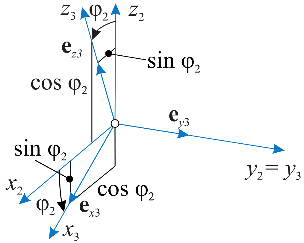
Fig. 19 Elementary rotation around axis \(\mathbf{ y}_2\).

Finally, a rotation around \({\mathbf{e}}_{z3}\) with angle \(\varphi_3\) would give similarly,

\[\LU{34}{\Rot} = \left[ \LUR{3}{{\mathbf{e}}}{x4} \;\; \LUR{3}{{\mathbf{e}}}{y4} \;\; \LUR{3}{{\mathbf{e}}}{z4} \right] = \mr{c \varphi_3}{-s \varphi_3}{0} {s \varphi_3}{c \varphi_3}{0} {0}{0}{1} .\]

Linearized rotations

In this case we can interpret the small rotations as a constant angular velocity over small time \(\Delta t\), \({\mathbf{t}}arphi = \Delta t \cdot \tomega\), which results in

\[{\mathbf{r}}_1^\prime= {\mathbf{r}}_1 + \Delta t \cdot (\tomega \times {\mathbf{r}}_1) = ({\mathbf{I}} + \tilde {\mathbf{t}}arphi) {\mathbf{r}}_1\]

Leading to the linearized rotation matrix

\[\Rot_\mathrm{lin} = {\mathbf{I}} - \tilde {\mathbf{t}}arphi\]

Alternatively, using linearized rotations \({\mathbf{t}}arphi = [\varphi_1,\;\varphi_2,\;\varphi_3]\tp\), with \(|{\mathbf{t}}arphi| \ll 1\), we can approximate \(\sin \varphi_1\) as:

\[\sin \varphi_1 = \varphi_1 - \frac{\varphi_1^3}{3!} + \frac{\varphi_1^5}{5!} - ... \approx \varphi_1\]

Similarly, we can approximate \(\cos \varphi_1 \approx 1\). This immediately gives a linearization for elementary rotations – where we observe that contributions for each axis can be added.

The axis-angle representation (see later) leads to the same result by linearization of the Rodrigues formula,

\[\Rot({\mathbf{u}}, \varphi) \approx {\mathbf{I}} + \tilde {\mathbf{u}} \varphi, \quad \Rot\tp \approx {\mathbf{I}} - \tilde {\mathbf{u}} \varphi\]

in which \(\varphi\) represents the infinitesimal angle and \({\mathbf{u}}\) is the rotation axis.

Note: whenever you would like to work with linearized rotations, or if you do not know the sequence of small rotations, still do not use the linearized formula as it gives immediately rotation matrices without strict orthogonality and determinant of 1. In order to avoid computational problems, use for example RotationVector2RotationMatrix(phi) to compute a consistent rotation matrix based on the matrix exponential.

Active and passive rotations

It is important to distinguish two fundamentally different concepts of rotations. There is the active rotation, which can be represented by a coordinate-free relation,

(16)\[{\mathbf{v}}^\prime = \Rot {\mathbf{v}}\]

in which a vector \({\mathbf{v}}\) is actively rotated into a new configuration \({\mathbf{v}}^\prime\) using a rotation tensor \(\Rot\). Eq. (16) can be represented in any coordinate system, but keeping it fixed.

Furthermore, we denote a passive rotation as a coordinate transformation, as used many times before,

\[\LU{1}{{\mathbf{v}}} = \LU{12}{\Rot} \LU{2}{{\mathbf{v}}}\]

in which the vector \({\mathbf{v}}\) is not changed at all, but only its coordinates are represented in two different coordinate systems.

While passive rotations (and homogeneous transformations) are used, e.g., to compute current positions of body-attached points through several relative coordinate systems, active rotations can represent the rotations from one time step to the next one.

Successive rotations

The successive application of rotation matrices is non-commutative. An exception is the planar case, i.e., all rotations occur around the same axis. Specifically, we see that for successive rotations, the following must be considered:

\[{\mathbf{A}}_2 {\mathbf{A}}_1 {\mathbf{v}} \neq {\mathbf{A}}_1 {\mathbf{A}}_2 {\mathbf{v}} .\]

As an example, we consider in Figure Successive rotations are not commutative. the different order of rotations of a block.

Fig. 20 Successive rotations are not commutative.

In Fig. 20a, the block shown is first rotated 90° about the \(\mathbf{e}_2\) axis and then 90° about the \(\mathbf{e}_3\) axis. In Figure Successive rotations are not commutative.b, the same rotations are applied in reverse order, i.e., the block is first rotated 90° about the \(\mathbf{e}_3\) axis and then 90° about the \(\mathbf{e}_2\) axis. It is immediately apparent that the resulting orientation of the block is different in both cases.

Finally, it should be noted that there are two different types of successive rotations. In the first variant, also known as the single-frame method, the same reference frame is chosen for each rotation. This variant is best understood in the active rotation of vectors, where these rotations always take place, for example, in the global reference system.

In the second variant, also known as the multi-frame method, a new reference frame created by the preceding rotation is used for each rotation. This variant can be illustrated by applications in robotics (e.g., articulated arm robots), where (passive) rotations of the reference systems of the robot’s respective arms occur, with each rotation taking place in the reference system of the preceding arm.

Rotation tensor: axis-angle representation

In the following, we will elaborate the rotation tensor, inherently linked to the axis-angle representation. Note that the rotation axis times the angle is denoted as rotation vector throughout.

Considering Euler’s theorem on rotations, we assume a transformation

\[{\mathbf{r}}_0 \ra {\mathbf{r}}(t)\]

which purely follows from a rotation. This transformation thus can be represented by a rotation axis \({\mathbf{u}}\) and an angle \(\varphi(t)\),

\[({\mathbf{u}}(t), \, \varphi(t))\]

both of them given in a coordinate-free manner. We may therefore conclude

\[{\mathbf{r}}(t)=\Rot(t) \, {\mathbf{r}}_0 \qquad \text{with} \qquad \Rot(t)=\Rot({\mathbf{u}}(t),\varphi(t))\]

Fig. 21 Rotation of a vector \(\mathbf{ r}_0\) by means of the angle-axis tuple \((\mathbf{ u}(t), \, \varphi(t))\).

Using Fig. 21, we may now consider relations of the two frames \(({\mathbf{e}}_{x0},\,{\mathbf{e}}_{y0},\,{\mathbf{e}}_{z0})\) and \(({\mathbf{e}}_{x1},\,{\mathbf{e}}_{y1},\,{\mathbf{e}}_{z1})\), solely defined by the angle-axis \(({\mathbf{u}}(t), \, \varphi(t))\) relation.

Fig. 22 Relations for derivation of rotation tensor and Rodrigues’ formula.

According to Fig. 22, we may split the vector \({\mathbf{r}}\), which has the length \(r = \vert {\mathbf{r}} \vert\), into

\[{\mathbf{r}}= c_1 {\mathbf{e}}_1 + c_2 {\mathbf{e}}_2 + c_3 {\mathbf{e}}_3\]

with the unit vectors given as

\[{\mathbf{e}}_1 = \frac{{\mathbf{r}}_0 - {\mathbf{u}}({\mathbf{u}}^{\mathrm{T}} {\mathbf{r}}_0)}{r \sin \delta}, \quad {\mathbf{e}}_2 = \frac{\tilde{{\mathbf{u}}} {\mathbf{r}}_0}{r \sin \delta}, \quad \mathrm{and} \quad {\mathbf{e}}_3 = {\mathbf{u}} .\]

The coefficients can be calculated as follows,

\[c_1 = r \sin \delta \cos \varphi, \quad c_2 = r \sin \delta \sin \varphi, \quad \mathrm{and} \quad c_3 = r \cos \delta\]

Putting everything together gives

\[{\mathbf{r}} = \cos \varphi \, {\mathbf{r}}_0 + \sin \varphi \, \tilde{{\mathbf{u}}} \, {\mathbf{r}}_0 + (1 - \cos \varphi) \, {\mathbf{u}} \, ({\mathbf{u}}\tp \, {\mathbf{r}}_0)\]

From the relation \({\mathbf{r}} = \Rot({\mathbf{u}} ,\varphi) {\mathbf{r}}_0\), we can reinterpret the rotation tensor \(\Rot\)

\[\Rot({\mathbf{u}} ,\varphi) = \cos \varphi \, {\mathbf{I}} + \sin \varphi \, \tilde{{\mathbf{u}}} + (1-\cos \varphi) \, {\mathbf{u}} \, {\mathbf{u}}\tp\]

With the additional relations

\[{\mathbf{u}} \, {\mathbf{u}}\tp=\tilde{\mathbf{u}} \, \tilde{\mathbf{u}} +({\mathbf{u}}\tp {\mathbf{u}}) {\mathbf{I}} \quad \mathrm{and} \quad {\mathbf{u}}\tp {\mathbf{u}} = 1\]

we finally obtain

\[\Rot({\mathbf{u}} ,\varphi) = {\mathbf{I}} + \sin \varphi \, \tilde{{\mathbf{u}}} + (1-\cos \varphi) \, \tilde{{\mathbf{u}}} \, \tilde{{\mathbf{u}}}\]

which is also known as the Rodrigues formula for rotations. While this formula is coordinate-free, it may be represented in any coordinate system, such as

\[\LU{0}{{\mathbf{r}}}(t)=\LU{0}{\Rot}(t) \, \LUR{0}{{\mathbf{r}}}{0} \qquad \text{with} \qquad \LU{0}{\Rot}(t)=\Rot(\LU{0}{{\mathbf{u}}}(t),\varphi(t))\]

Rotation vector

Using the rotation vector \({\mathbf{v}}_\mathrm{rot} = \varphi\cdot {\mathbf{u}}\) and \(\varphi = |{\mathbf{v}}_\mathrm{rot}|\), another representation of the rotation tensor follows as

\[\Rot({\mathbf{u}} ,\varphi) = {\mathbf{I}} + \frac{\sin \varphi}{\varphi} \tilde{\mathbf{v}}_\mathrm{rot} + \frac{(1-\cos \varphi)}{\varphi^2} \, \tilde{\mathbf{v}}_\mathrm{rot} \, \tilde{\mathbf{v}}_\mathrm{rot}\]

Note, that we inherently assume that \(\varphi \in [0,\pi]\). In Exudyn, there are the following functions and items related to the rotation vector and the axis-angle representation:

• NodeRigidBodyRotVecLG: A 3D rigid body node based on rotation vector and Lie group methods; can be used for explicit integration methods, not leading to singularities when integrating with Lie-group methods

• RotationVector2RotationMatrix: computes the rotation matrix from a given rotation vector \({\mathbf{v}}_\mathrm{rot}\)

• RotationMatrix2RotationVector: computes the rotation vector \({\mathbf{v}}_\mathrm{rot}\) from a given rotation matrix, based on a reconstruction of Euler parameters

• ComputeRotationAxisFromRotationVector: computes the rotation axis \({\mathbf{u}}\) from the rotation vector by using \(\varphi = |{\mathbf{v}}_\mathrm{rot}|\)

Note the following properties of the rotation tensor:

• The axis-angle representations \(({\mathbf{u}}, \varphi)\) and \((-{\mathbf{u}}, -\varphi)\) represent the same tensor \(\Rot({\mathbf{u}},\varphi)=\Rot(-{\mathbf{u}},-\varphi)\)

• The rotation tensor \(\Rot\) is orthogonal, i.e., \(\Rot\tp \, \Rot = {\mathbf{E}}\).

• The inverse rotation tensor \(\Rot^{-1} = \Rot\tp\) is represented by the identical axis-angle tuples \(({\mathbf{u}}, -\varphi)\) and \((-{\mathbf{u}}, \varphi)\), leading to \({\mathbf{r}}_0=\Rot({\mathbf{u}}, -\varphi) {\mathbf{r}}\).

• We furthermore not the identities: \(\Rot({\mathbf{u}}, -\varphi) \equiv \Rot(-{\mathbf{u}}, \varphi) \equiv \Rot\tp ({\mathbf{u}}, \varphi)\)

• The rotation axis is invariant to the rotation: \(\Rot({\mathbf{u}}, \varphi) {\mathbf{u}} = {\mathbf{u}}\)

Euler angles: Tait-Bryan angles

In the following section, we discuss rotation matrices built by Tait-Bryan angles, which are consecutive \(xyz\)-rotations. Note that there are many other representations of Euler angles, however, they are not implemented or used in Exudyn. The output variable Rotation gives Tait-Bryan angles, which is why it is important to define their properties.

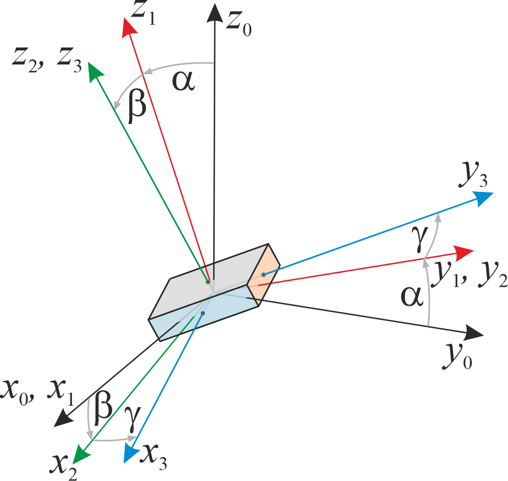
Fig. 23 Definition of Tait-Bryan angles.

The transformation given by Tait-Bryan angles \((\alpha,\beta,\gamma)\) follows from three successive rotations,

\[\LU{0}{{\mathbf{r}}} = \LU{01}{\Rot}(\alpha) \, \LU{12}{\Rot}(\beta) \, \LU{23}{\Rot}(\gamma) \, \LU{3}{{\mathbf{r}}} \quad \mathrm{and} \quad \LU{0}{{\mathbf{r}}} = \LU{03}{\Rot}(\alpha,\beta,\gamma) \, \LU{3}{{\mathbf{r}}}\]

The Tait-Bryan rotation matrix is thus defined as

\[\LU{03}{\Rot}(\alpha,\beta,\gamma) = \mr{\co\beta \,\co\gamma}{-\co\beta\,\si\gamma}{\si\beta} {\co \alpha \,\si \gamma + \si \alpha \,\si \beta \,\co \gamma}{\co \alpha \,\co\gamma-\si\alpha\,\si\beta\,\si\gamma}{-\si\alpha\,\co\beta} {\si\alpha\,\si\gamma-\co\alpha\,\si\beta\,\co\gamma}{\si\alpha\,\co\gamma+\co\alpha\,\si\beta\,\si\gamma}{\co\alpha\,\co\beta}\]

While not fully obvious from the latter equations, we note that there is a singularity at \(|\beta| = \frac{\pi}{2}\), which causes any computations to stall whenever getting close enough to this value.

It is also possible to reconstruct Tait-Bryan angles from a given rotation matrix. Assume, we have the rotation matrix \(\LU{03}{\Rot}=(A_{ij})\). There are two solutions for \(\beta\) which follow from

\[\cos \beta = \pm \sqrt{1-A_{13}^2}, \quad \mathrm{and} \quad \sin \beta = A_{13}\]

For beta fulfilling \(|\beta| \ne \frac{\pi}{2}\), we can uniquely compute \(\gamma\) and \(\alpha\),

\[\cos \gamma = \frac{A_{11}}{\cos \beta}, \quad \sin \gamma = - \frac{A_{12}}{\cos \beta}, \quad \cos \alpha = \frac{A_{33}}{\cos \beta}, \quad \mathrm{and} \quad \sin \alpha = - \frac{A_{23}}{\cos \beta} .\]

Note that improvements are possible using the \(\mathrm{atan2}()\) function. We can finally resolve non-uniqueness by restricting \(\beta\) within the range \(-\frac{\pi}{2} < \beta < \frac{\pi}{2}\).

Tait-Bryan angles: angular velocity vector

Angular velocities are essential for the formulation of equations of motion of rigid bodies, for constraints and for evaluation. Therefore, basic relations are shown for Tait-Bryan angles, in particular the velocity transformation matrix \({\mathbf{G}}_{TB}\).

The angular velocity vector \(\omega\) can either be computed from the basic relation \(\dot \Rot = \tilde \omega \Rot\), which however involves many trigonometric terms, or from partial angular velocities, being part of the co-rotated rotation axes. With the latter approach, we see that

\[\tomega_{30}=\dot{\alpha} {\mathbf{e}}_{x0}+\dot{\beta} {\mathbf{e}}_{y1}+\dot{\gamma} {\mathbf{e}}_{z2} \quad \text{or} \quad \tomega_{30}=\underbrace{[{\mathbf{e}}_{x0} \quad {\mathbf{e}}_{y1} \quad {\mathbf{e}}_{z2}]}_{{\mathbf{G}}_{TB}} \vr{\dot{\alpha}}{\dot{\beta}}{\dot{\gamma}}\]

We can now evaluate this equation in frame \(\mathcal{F}_0\) with \(\tbeta=[\alpha\;\beta\;\gamma]\tp\), written as

\[\LUR{0}{\tomega}{30}=\underbrace{[\LUR{0}{{\mathbf{e}}}{x0} \quad \LUR{0}{{\mathbf{e}}}{y1} \quad \LUR{0}{{\mathbf{e}}}{z2}]}_{\LUR{0}{{\mathbf{G}}}{TB}} \vr{\dot{\alpha}}{\dot{\beta}}{\dot{\gamma}} = \LUR{0}{{\mathbf{G}}}{TB}(\tbeta) \dot{\tbeta} .\]

Evaluating the consecutive rotations, we find the respective unit vectors as

\[\LUR{0}{{\mathbf{e}}}{x0} = \vr{1}{0}{0}, \quad \LUR{0}{{\mathbf{e}}}{y1} = \vr{0}{\text{c} \alpha}{\text{s} \alpha}, \quad \mathrm{and} \quad \LUR{0}{{\mathbf{e}}}{z2} = \vr{\text{s} \beta}{-\text{s} \alpha \text{c} \beta}{\text{c} \alpha \text{c} \beta} .\]

which results in the relations for the (global) angular velocity vector

(17)\[\vr{\LUR{0}{\omega}{30x}}{\LUR{0}{\omega}{30y}}{\LUR{0}{\omega}{30z}} = \mr{1}{0} {\text{s} \beta} {0}{\text{c} \alpha} {-\text{s} \alpha \text{c} \beta} {0}{\text{s} \alpha} {\text{c} \alpha \text{c} \beta} \vr{\dot{\alpha}}{\dot{\beta}}{\dot{\gamma}}\]

The matrix \(\LUR{0}{{\mathbf{G}}}{TB}\) is used to compute partial derivatives of the angular velocity vector w.r.t. rotations. However, it is also used to project torques and angular velocities into a space given by \({\mathbf{G}}_{TB}^\mathrm{T}\) (which is indeed not equivalent to \({\mathbf{G}}_{TB}^{-1}\), but gives a symmetric mass matrix – see the equations of motion for the rigid body).

The inverse relation between \(\dot \tbeta\) and \(\LUR{0}{\tomega}{30}\) gives

(18)\[\vr{\dot{\alpha}}{\dot{\beta}}{\dot{\gamma}} = \frac{1}{\text{c} \beta} \mr{\text{c} \beta}{\text{s} \alpha \, \text{s} \beta}{-\text{c} \alpha \, \text{s} \beta}{0}{\text{c} \alpha \, \text{c} \beta}{\text{s} \alpha \text{c} \beta}{0}{-\text{s} \alpha}{\text{c} \alpha} \vr{\LUR{0}{\omega}{30x}}{\LUR{0}{\omega}{30y}}{\LUR{0}{\omega}{30z}}\]

or in compact form

\[\dot{\tbeta} = \LURU{0}{{\mathbf{G}}}{TB}{-1}(\tbeta) \LUR{0}{\tomega}{30}\]

We again see that for the case \(\vert \beta \vert = \pi/2\) the matrix\(\LUR{0}{{\mathbf{G}}}{TB}\) becomes singular, and Eq. (18) cannot be resolved for \(\dot{\tbeta}\)!

Finally, we also provide the relations of \(\tomega_{30}\) in body-fixed (local) coordinates \(\mathcal{F}_3\), which are frequently used in the implementation,

\[\vr{\LUR{3}{\omega}{30x}}{\LUR{3}{\omega}{30y}}{\LUR{3}{\omega}{30z}} = \mr{\text{c} \beta \, \text{c} \gamma}{\text{s} \gamma}{0}{-\text{c} \beta \, \text{s} \gamma}{\text{c} \gamma}{0}{\text{s} \beta}{0}{1} \vr{\dot{\alpha}}{\dot{\beta}}{\dot{\gamma}} ,\]

which reads in compact form (\(\LUR{3}{{\mathbf{G}}}{TB} = \LUR{b}{{\mathbf{G}}}{TB}\)),

\[\LUR{3}{\tomega}{30} = \LUR{3}{{\mathbf{G}}}{TB}(\tbeta) \dot{\tbeta}\]

In Exudyn, there are the following functions and items related to Tait-Bryan angles:

• NodeRigidBodyRxyz: A 3D rigid body node based on Tait-Bryan angles

• RotXYZ2RotationMatrix: computes the rotation matrix from given Tait-Bryan angles

• RotationMatrix2RotXYZ: computes Tait-Bryan angles from a given rotation matrix

• RotXYZ2G: computes the matrix \(\LU{0}{{\mathbf{G}}}\) relating time derivatives of Tait-Bryan angles to the (global) angular velocity vector

• RotXYZ2Glocal: computes the matrix \(\LU{b}{{\mathbf{G}}}\) relating time derivatives of Tait-Bryan angles to the (local, body-fixed) angular velocity vector

Euler parameters and unit quaternions

As one of the most important forms of rotational parameters for multibody systems, the 4 Euler parameters are introduced. They can be mathematically represented as unit quaternions and provide particularly simple expressions and equations of motion, albeit at the expense of an additional constraint.

The Euler parameters are defined as

(19)\[\underline{{\mathbf{p}}}=\vp{p_{\mathrm{s}}}{{\mathbf{p}}}=\vp{\cos \frac \varphi 2}{{\mathbf{u}} \, \sin \frac\varphi 2} \quad \text{bzw.} \quad \underline{{\mathbf{p}}}=\vfour{p_{\mathrm{s}}}{p_x}{p_y}{p_z}=\vfour{\cos \frac\varphi 2}{u_x \, \sin \frac\varphi 2}{u_y \, \sin \frac\varphi 2}{u_z \, \sin \frac\varphi 2}\]

Here, \(p_s=\cos \frac\varphi 2\) is the scalar part and \({\mathbf{p}} = {\mathbf{u}} \, \sin \frac\varphi 2\) is the vector part of the Euler parameters \(\underline{{\mathbf{p}}}\). The four Euler parameters \(\underline{{\mathbf{p}}}\) are subject to the normalization condition

\[\phi(\underline{{\mathbf{p}}}) \equiv p_s^2+p_x^2+p_y^2+p_z^2-1=0 \quad \mathrm{or} \quad p_s^2 +{\mathbf{p}}\tp \, {\mathbf{p}} -1 = 0 .\]

First, the following trigonometric transformations are introduced,

\[\cos \varphi = 2 \cos^2\frac{\varphi}{2} -1, \quad \sin \varphi = 2 \sin \frac \varphi 2 \cos \frac \varphi 2, \quad 1-\cos \varphi = 2 \sin^2 \frac{\varphi}{2} .\]

When these are substituted into the rotation tensor using Eq. (19), it follows

\[\Rot(\underline{{\mathbf{p}}})=(2 p_{\mathrm{s}}^2-1) \, {\mathbf{E}} + 2 p_{\mathrm{s}} \, \tilde{{\mathbf{p}}} + 2 \, {\mathbf{p}} \, {\mathbf{p}}\tp .\]

Euler parameters can initially be expressed in the global reference frame \(\mathcal{F}_0\),

\[\LU{0}{\underline{{\mathbf{p}}}}=\vp{p_{\mathrm{s}}}{\LU{0}{{\mathbf{p}}}}=\vp{\cos \frac\varphi 2}{\LU{0}{{\mathbf{u}}} \, \sin \frac{\varphi} {2}} .\]

Thus, the coordinate representation of the rotation tensor is given by

(20)\[\Rot(\LU{0}{\underline{{\mathbf{p}}}}) = 2 \LU{0}{\mr{\ps^2+p_x^2-\frac 1 2}{p_x p_y-\ps p_z}{p_x p_z+\ps p_y} {p_x p_y+\ps p_z}{\ps^2+p_y^2-\frac 1 2}{p_y p_z-\ps p_x} {p_x p_z-\ps p_y}{p_y p_z+\ps p_x}{\ps^2+p_z^2-\frac{1}{2} }} = \LU{01}{\Rot}\]

Note that the axis of rotation is invariant to the rotation, \(\LU{0}{{\mathbf{u}}} = \LU{1}{{\mathbf{u}}}\), thus \(\LU{0}{\underline{{\mathbf{p}}}} = \LU{1}{\underline{{\mathbf{p}}}}\)Due to the ambiguity \(\Rot(\underline{{\mathbf{p}}}) = \Rot(-\underline{{\mathbf{p}}})\), the scalar part of the Euler parameters is usually normalized, i.e., \(p_s \ge 0\).

The careful reader may observe that matrix \(\Rot\) in Eq. (20) is not identical to the implementation in Exudyn. This is true, because there is always an alternative formulation for the diagonal terms by adding the normalization condition times a factor.

Quaternion operations

Calculations with Euler parameters are efficiently performed through the rules of quaternion algebra. Active perspective as vector rotation: The rotation of vector \({\mathbf{r}}_0\) into \({\mathbf{r}}(t)\),

(21)\[\LU{0}{{\mathbf{r}}}(t)=\LU{0}{\Rot}(t) \, \LUR{0}{{\mathbf{r}}}{0} \quad \text{mit} \quad \LU{0}{\Rot}(t)= \Rot(\LU{0}{{\mathbf{u}}}(t), \varphi (t))\]

is formulated using the quaternion \(\LU{0}{\underline{{\mathbf{p}}}}=\underline{{\mathbf{p}}}(\LU{0}{{\mathbf{u}}}, \varphi)\) and its conjugate \(\myoverline{\underline{{\mathbf{p}}}}\) with the help of the double quaternion product (operator \(\circ\)),

\[\LU{0}{\underline{{\mathbf{r}}}}(t) = \LU{0}{\underline{{\mathbf{p}}}}(t) \, \circ \, \LUR{0}{\underline{{\mathbf{r}}}}{0} \, \circ \, \LU{0}{\underline{\myoverline{{\mathbf{p}}}}}(t) ,\]

or in short form,

\[\vp{0}{\LU{0}{{\mathbf{r}}}(t)}=\vp{p_{\mathrm{s}}(t)}{\LU{0}{{\mathbf{p}}}(t)} \, \circ \, \vp{0}{\LUR{0}{{\mathbf{r}}}{0}} \, \circ \, \vp{p_{\mathrm{s}}(t)}{-\LU{0}{{\mathbf{p}}}(t)} .\]

With the multiplication rule for quaternions, the scalar part yields \(0=0\) and the vector part the vector rotation (21). For multiple rotations, we have

\[\LUR{0}{\underline{{\mathbf{r}}}}{2}=\LUR{0}{\underline{{\mathbf{p}}}}{2} \circ \LUR{0}{\underline{{\mathbf{p}}}}{1} \circ \LUR{0}{\underline{{\mathbf{r}}}}{0} \circ \LUR{0}{\myoverline{\underline{{\mathbf{p}}}}}{1} \circ \LUR{0}{\myoverline{\underline{{\mathbf{p}}}}}{2} .\]

Given two quaternions

\[\underline{{\mathbf{a}}} = a_\mathrm{s} + \mathrm{i}\, a_x + \mathrm{j}\, a_y + \mathrm{k}\, a_z, \quad \mathrm{and} \quad \underline{{\mathbf{b}}} = b_\mathrm{s} + \mathrm{i}\, b_x + \mathrm{j}\, b_y + \mathrm{k}\, b_z ,\]

we provide two important rules of quaternion algebra, which is the sum,

\[\underline{{\mathbf{c}}} = \underline{{\mathbf{a}}} + \underline{{\mathbf{b}}} \quad \ra \quad \vp{c_\mathrm{s}}{{\mathbf{c}}} = \vp{a_\mathrm{s}}{{\mathbf{a}}} + \vp{b_\mathrm{s}}{{\mathbf{b}}} = \vp{a_\mathrm{s} + b_\mathrm{s}}{{\mathbf{a}} + {\mathbf{b}}} ,\]

and the multiplication

\[\underline{{\mathbf{c}}} = \underline{{\mathbf{a}}} \circ \underline{{\mathbf{b}}} \neq \underline{{\mathbf{b}}} \circ \underline{{\mathbf{a}}} \quad \ra \quad \vp{c_\mathrm{s}}{{\mathbf{c}}} = \vp{a_\mathrm{s}}{{\mathbf{a}}} \circ \vp{b_\mathrm{s}}{{\mathbf{b}}} = \vp{a_\mathrm{s} b_\mathrm{s} - {\mathbf{a}}^\mathrm{T} {\mathbf{b}}}{a_\mathrm{s}{\mathbf{b}} + b_\mathrm{s}{\mathbf{a}} + \tilde {\mathbf{a}} {\mathbf{b}}} .\]

Angular velocity vector

To derive the angular velocity from Euler parameters, there are both the possibilities of deriving the rotation matrix with respect to time and directly deriving the angular velocity from Euler parameters.

For an infinitesimal rotation \(\dd \psi\), the quaternion follows

\[\underline{{\mathbf{p}}}({\mathbf{e}}, \dd \psi) = \vp{\cos \frac{\dd \psi}{2}}{{\mathbf{e}} \sin \frac{\dd\psi}{2}} \approx \vp{1}{{\mathbf{e}} \frac{\dd\psi}{2}}\]

from which we conclude that from \(\underline{{\mathbf{p}}}({\mathbf{e}}, \dd \psi) \, \circ \, \underline{{\mathbf{p}}}(t) = \underline{{\mathbf{p}}}(t) + \dd\underline{{\mathbf{p}}}\) and thus \(\dd\underline{{\mathbf{p}}} = \vp{0}{{\mathbf{e}} \frac{\dd\psi}{2}}\). Dividing by \(\dd t\) and with the angular velocity \(\tomega_{10} = {\mathbf{e}} \, \dot \psi\), it follows

\[\vp{\dot \ps}{\LLdot{0}{{\mathbf{p}}}{}} = \frac{1}{2} \vp{0}{\tomega_{10} } \circ \vp{\ps}{{\mathbf{p}}}\]

or in short form

\[\LU{0}{\underline{\dot {\mathbf{p}}}} = \frac{1}{2} \underline{\tomega}_{10} \circ \underline{{\mathbf{p}}}\]

With the quaternion product in matrix notation, it follows

\[\vp{\dot \ps}{\LU{0}{\dot{\mathbf{p}}}{}} = \frac{1}{2} \mp{\ps}{-{\mathbf{p}}^\mathrm{T}}{{\mathbf{p}}}{\ps {\mathbf{E}} - \tilde {\mathbf{p}}} \vp{0}{\tomega_{10} }\]

or with the matrix \(\underline{{\mathbf{P}}}\) it can be written as

\[\LU{0}{\underline{\dot {\mathbf{p}}}}{} = \frac{1}{2} {\underline{{\mathbf{P}}}}({\mathbf{p}}) \underline{\tomega}_{10}\]

This form can be represented in global coordinates due to \({\underline{{\mathbf{P}}}}^{-1} = {\underline{{\mathbf{P}}}}\tp\) as

\[\vp{0}{\LU{0}{\tomega}_{10} } = 2 \mp{\ps}{\LU{0}{{\mathbf{p}}}^\mathrm{T}}{-\LU{0}{{\mathbf{p}}}}{\ps {\mathbf{E}} + \LU{0}{\tilde {\mathbf{p}}}} \, \vp{\dot \ps}{\LLdot{0}{{\mathbf{p}}}{}}\]

Thus, the velocity transformation follows to

\[\LUR{0}{{\mathbf{G}}}{EP} = \left[-2\LU{0}{{\mathbf{p}}}, \; 2\ps {\mathbf{E}} + 2\LU{0}{\tilde {\mathbf{p}}}\right]\]

as a matrix with 3 rows and 4 columns. With \(\LUR{0}{{\mathbf{G}}}{EP}\), the angular velocity vector can be conveniently calculated,

\[\LU{0}{\tomega}_{10} = \left[-2\LU{0}{{\mathbf{p}}}, \; 2\ps {\mathbf{E}} + 2\LU{0}{\tilde {\mathbf{p}}}\right] \, \LU{0}{\underline{\dot {\mathbf{p}}}}\]

In Exudyn, there are the following functions and items related to Euler parameters:

• NodeRigidBodyEP: A 3D rigid body node based on Euler parameters

• EulerParameters2RotationMatrix: computes the rotation matrix from given Euler parameters

• RotationMatrix2EulerParameters: computes Euler parameters from a given rotation matrix

• EulerParameters2G: computes the matrix \(\LUR{0}{{\mathbf{G}}}{EP}\) relating time derivatives of Euler parameters to the (global) angular velocity vector

• EulerParameters2Glocal: computes the matrix \(\LUR{b}{{\mathbf{G}}}{EP}\) relating time derivatives of Euler parameters to the (local, body-fixed) angular velocity vector