Overview on Exudyn

This section provides a general overview on important parts of Exudyn. It is recommended to read these parts as it alleviates your life in creating models, understanding the behavior of the system and resolving errors.

Module structure

This section will show:

• Overview of modules

• Conventions: dimension of nodes, objects and vectors

• Coordinates: reference coordinates and displacements

• Nodes, Objects, Markers and Loads

For an introduction to the solvers, see Solvers.

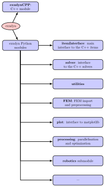
Fig. 1 Overview on Exudyn C++ and Python modules

Overview of modules

Currently, the Exudyn module structure is split into a C++ core part and a set of Python parts, see Fig. 1.

• C++ parts, see Fig. 2 and Fig. 3:

  • exudyn: on this level, there are just very few functions: SystemContainer(), SC.renderer.Start(), SC.renderer.Stop(), SolveStatic(...), SolveDynamic(...), … as well as system and user variable dictionaries exudyn.variables and exudyn.sys

  • config, special: substructures for configuration (global settings) and special settings; use e.g. exudyn.config.outputPrecision=4

  • symbolic: tools for symbolic computation in user functions (speedup!)

  • SystemContainer: contains the systems (most important), solvers (static, dynamics, …), visualization settings

  • MainSystem mbs: mbs created with mbs = SC.AddSystem(), this structure contains everything that defines a solvable multibody system; a large set of nodes, objects, markers, loads can added to the system, see Items reference manual;

  • mbs.systemData: contains the initial, current, visualization, … states of the system and holds the items, see Fig. 3

  • SimulationSettings: contains the systems (most important), solvers (static, dynamics, …), visualization settings

• Python parts (this list is continuously extended, see Python Utility Functions):

  • exudyn.artificialIntelligence: interface to stablebaselines, interface to pytorch training (coming soon)

  • exudyn.basicUtilities: contains basic helper classes, without importing numpy

  • exudyn.beams: helper functions for creation of beams along straight lines and curves, sliding joints, etc.

  • exudyn.graphics: provides some basic drawing utilities, definition of colors and basic drawing objects (including STL import); rotation/translation of graphicsData objects

  • exudyn.interactive: helper classes to create interactive models (e.g. for teaching or demos)

  • exudyn.itemInterface: contains the interface, which transfers Python classes (e.g., of a NodePoint) to dictionaries that can be understood by the C++ module

  • exudyn.FEM: everything related to finite element import and creation of model order reduction flexible bodies

  • exudyn.lieGroupBasics: a collection of Python functions for Lie group methods (SO3, SE3, log, exp, Texp, …)

  • exudyn.misc.mainSystemExtensions: mapping of some functions to MainSystem (mbs)

  • exudyn.physics: containing helper functions, which are physics related such as friction

  • exudyn.plot: contains PlotSensor(…), a very versatile interface to matplotlib and other valuable helper functions

  • exudyn.processing: methods for optimization, parameter variation, sensitivity analysis, etc.

  • exudyn.rigidBodyUtilities: contains important helper classes for creation of rigid body inertia, rigid bodies, and rigid body joints; includes helper functions for rotation parameterization, rotation matrices, homogeneous transformations, etc.

  • exudyn.robotics: submodule containing several helper modules related to manipulators (robotics, robotics.models), mobile robots (robotics.mobile), trajectory generation (robotics.motion), etc.

  • exudyn.signalProcessing: filters, FFT, etc.; interfaces to scipy and numpy methods

  • exudyn.solver: functions imported when loading exudyn, containing main solvers

  • exudyn.utilities: constains helper classes in Python and includes Exudyn main modules basicUtilities, rigidBodyUtilities, graphics, and itemInterface, which is recommended to be loaded at beginning of your model file in order to have most necessary functionality at hand

Fig. 2 Overview on Exudyn C++ module

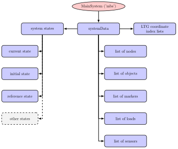
Fig. 3 Overview of systemData

SystemData connects items, states and stores the LTG. Note that access to items is provided via functions in MainSystem.

Conventions: items, indexes, coordinates

In this documentation, we will use the term item to identify nodes, objects, markers, loads and sensors:

item \(\in\) {node, object, marker, load, sensor}

Indexes: arrays and vectors starting with 0: As known from Python, all indexes of arrays, vectors, matrices, … are starting with 0. This means that the first component of the vector v=[1,2,3] is accessed with v[0] in Python (and also in the C++ part of Exudyn ). The range is usually defined as range(0,3), in which ‘3’ marks the index after the last valid component of an array or vector.

Dimensionality of objects and vectors: 2D vs. 3D

As a convention, quantities in Exudyn are 3D, such as nodes, objects, markers, loads, measured quantities, etc. For that reason, we denote planar nodes, objects, etc. with the suffix 2D, but 3D objects do not get this suffix (There are some rare exceptions, such as Beam3D as the pure beam may easily lead to name space conflicts in Python).

Output and input to objects, markers, loads, etc. is usually given by 3D vectors (or matrices), such as (local) position, force, torque, rotation, etc. However, initial and reference values for nodes depend on their dimensionality. As an example, consider a NodePoint2D:

• referenceCoordinates is a 2D vector (but could be any dimension in general nodes)

• measuring the current position of NodePoint2D gives a 3D vector

• when attaching a MarkerNodePosition and a LoadForceVector, the force will be still a 3D vector

Furthermore, the local position in 2D objects is provided by a 3D vector. Usually, the dimensionality is given in the reference manual. User errors in the dimensionality will be usually detected either by the Python interface (i.e., at the time the item is created) or by the system-preprocessor

Items: Nodes, Objects, Loads, Markers, Sensors, …

In this section, the most important part of Exudyn are provided. An overview of the interaction of the items is given in Fig. 4

Fig. 4 Interaction of items in a multibody system

Note that both, bodies and connectors (including constraints) are – computational – objects. The arrows indicate, that, e.g., object 1 has node 1 and node 2 (indexes) and that marker 0 is attached to object 0, while load 0 uses marker 0 to apply the load. Sensors could additionally be attached to certain items.

Nodes

Nodes provide the coordinates (and the degrees of freedom) to the system. They have no mass, stiffness or whatsoever assigned. Without nodes, the system has no unknown coordinates. Adding a node provides (for the system unknown) coordinates. In addition we also need equations for every nodal coordinate – otherwise the system cannot be computed (NOTE: this is currently not checked by the preprocessor). In general, adding nodes and objects (e.g., to represent rigid bodies), leads to a redundant coordinate formulation. In order to determine the degree of freedom, you may use the Grübler-Kutzbach criterion. This can also be done numerically, using the function ComputeSystemDegreeOfFreedom, see the module exudyn.solver. Furthermore, minimal coordinates can be used for open tree systems, using ObjectKinematicTree.

Objects

Objects are ‘computational objects’ and they provide equations to your system. Objects often provide derivatives and have measurable quantities (e.g. displacement) and they provide access, which can be used to apply, e.g., forces. Some of this functionality is only available in C++, but not in Python.

Objects can be a:

• general object (e.g. a controller, user defined object, …; no example yet)

• body: has a mass or mass distribution; markers can be placed on bodies; loads can be applied; constraints can be attached via markers; bodies can be:

  • ground object: has no nodes

  • simple body: has one node (e.g. mass point, rigid body)

  • finite element and more complicated body (e.g. FFRF-object): has more than one node

• connector: uses markers to connect nodes and/or bodies; adds additional terms to system equations either based on stiffness/damping or with constraints (and Lagrange multipliers). Possible connectors:

  • algebraic constraint (e.g. constrain two coordinates: \(q_1 = q_2\))

  • classical joint

  • spring-damper or penalty constraint

Markers

Markers are interfaces between objects/nodes and constraints/loads. A constraint (which is also an object) or load cannot act directly on a node or object without a marker. As a benefit, the constraint or load does not need to know whether it is applied, e.g., to a node or to a local position of a body.

Typical situations are:

• Node – Marker – Load

• Node – Marker – Constraint (object)

• Body(object) – Marker – Load

• Body1 – Marker1 – Joint(object) – Marker2 – Body2

Loads

Loads are used to apply forces and torques to the system. The load values are static values. However, you can use Python functionality to modify loads either by linearly increasing them during static computation or by using the ‘mbs.SetPreStepUserFunction(…)’ structure in order to modify loads in every integration step depending on time or on measured quantities (thus, creating a controller).

Sensors

Sensors are only used to measure output variables (values) in order to simpler generate the requested output quantities. They have a very weak influence on the system, because they are only evaluated after certain solver steps as requested by the user.

Reference coordinates and displacements

Nodes usually have separated reference and initial quantities. Here, referenceCoordinates are the coordinates for which the system is defined upon creation. Reference coordinates are needed, e.g., for definition of joints and for the reference configuration of finite elements. In many cases it marks the undeformed configuration (e.g., with finite elements), but not, e.g., for ObjectConnectorSpringDamper, which has its own reference length.

Initial displacement (or rotation) values are provided separately, in order to start a system from a configuration different from the reference configuration. As an example, the initial configuration of a NodePoint is given by referenceCoordinates + initialCoordinates, while the initial state of a dynamic system additionally needs initialVelocities. See also Reference and current coordinates!

Note that commonly the OutputVariableType Coordinates returns coordinates without reference values, which are usually displacements (or changes in the rotation parameters), which is required if you are interested, e.g., in motion of finite element nodes. In contrast the OutputVariableType CoordinatesTotal returns (Since Exudyn1.9.25) the sum of reference and displacement (or rotation) coordinates for any configuration (e.g., current, initial or visualization).

Mapping between local and global coordinate indices

The LTG-index-mappings (local-to-global coordinate index mappings containing transformation from local object coordinate indices to global (system) coordinate indices; this is different for coordinate transformations!) between local coordinate indices, on node or object level, and global (=system) coordinate indices follows the following rules:

• LTG-index-mappings are computed during mbs.Assemble() and are not available before.

• Nodes own a global index which relates the local coordinates to global (system) coordinate. E.g., for a ODE2 node with node number i, this index can be obtained via the function mbs.GetNodeODE2Index(i).

• The order of global coordinates is simply following the node numbering. If we add three nodes NodePoint, the system will contain 9 coordinates, where the first triple (starting index 0) belongs to node 0, the second triple (starting index 3) belongs to node 1 and the third triple (starting index 6) belongs to node 2. After mbs.Assemble(), you can access the system coordinates via mbs.systemData.GetODE2Coordinates(), which returns a numpy array with 9 coordinates, containing the initial values provided in NodePoint (default: zero).

• Objects have their own LTG-index-mappings for their respective coordinate types. The ODE2 coordinates of an object j can be retrieved via mbs.systemData.GetObjectLTGODE2(j). For a body, these are the global ODE2 coordinates representing the body; for a connector, these are the coordinates to which the connector is linked (usually coordinates of two bodies); for a ground object, the LTG-index-mapping is empty; see also SystemData: Get object LTG coordinate mappings.

• Constraints create algebraic variables (Lagrange multipliers) automatically. For a constraint with object number k, the global index to algebraic variables (of AE-type) can be accessed via mbs.systemData.GetObjectLTGAE(k).